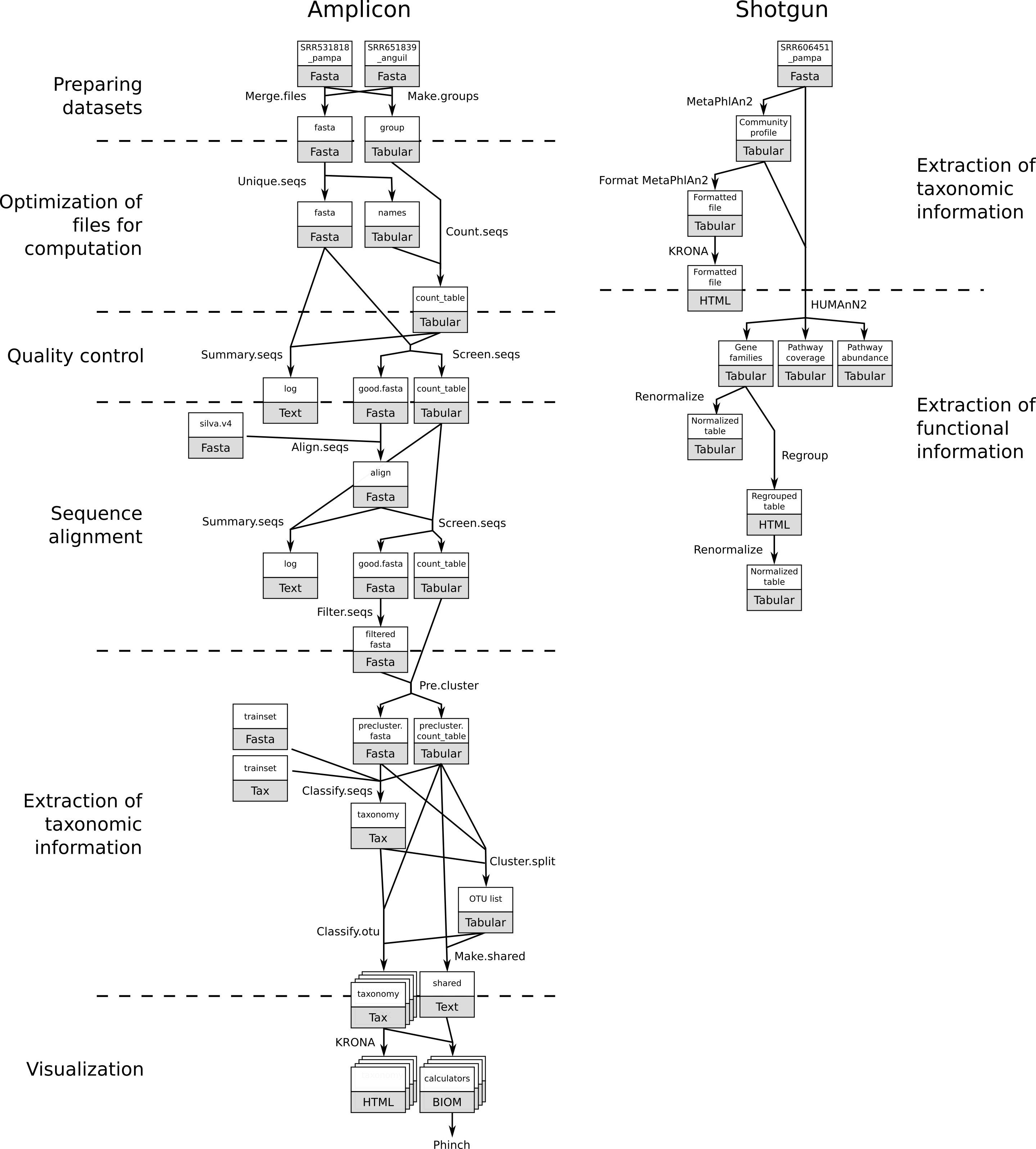
How to analyze metagenomics data? What information can be extracted of metagenomics data? What is the difference between amplicon and shotgun data? What are the difference in the analyses of amplicon and shotgun data?
In metagenomics, information about micro-organisms in an environment can be extracted with two main techniques:
In this lecture, we will introduce the two main types of analyses with their general principles and differences.
We will use two datasets (one amplicon and one shotgun) from the same project on the Argentinean agricultural pampean soils.
In this project, three different geographic regions that are under different types of land uses and two soil types (bulk and rhizospheric) were analyzed using shotgun and amplicon sequencing.
We will focus on data from the Argentina Anguil and Pampas Bulk Soil: the original study included one more geographical regions (Rascovan et al. 2013.)
Amplicon sequencing is a highly targeted approach for analyzing genetic variation in specific genomic regions. In the metagenomics fields, amplicon sequencing refers to capture and sequence of rRNA data in a sample. It can be 16S for bacteria or archea or 18S for eukaryotes.
The 16S rRNA gene has several properties that make it ideally suited to our purposes
With amplicon data, we can determine the micro-organisms from which the sequences in our sample are coming from. This is called taxonomic assignation. We try to assign sequences to taxons and then classify or extract the taxonomy in our sample.
https://zenodo.org/record/815875/files/SRR531818_pampa.fasta
https://zenodo.org/record/815875/files/SRR651839_anguil.fasta
We will perform a multisample analysis with mothur. To do this, we will merge all reads into a single file, and create a group file, indicating which reads belong to which samples.
Merge.files tool with the following parameters:
Make.group tool with the following parameters:
View the resulting datasets.
It contains two columns: the first contains the read names, the second contains the group (sample) name, in our case pampa or anguil.
Because we are sequencing many of the same organisms, we anticipate that many of our sequences are duplicates of each other.
Unique.seqs tool with the following parameters:
View the resulting datasets.
Unique.seqs tool outputs two files:
Question
Count.seqs tool with the following parameters:
Unique.seqsMake.groupView the resulting datasets.
The Count.seqs file keeps track of the number of sequences represented by each unique representative across multiple samples.
We will pass this file to many of the following tools to be used or updated as needed.
Summary.seqs tool with the following parameters:
Unique.seqsCount.seqs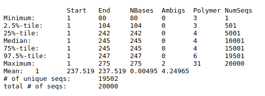
We will remove any sequences with ambiguous bases (maxambig parameter), homopolymer stretches of 9 or more bases (maxhomop parameter) and any reads longer than 275 bp or shorter than 225 bp.
Screen.seqs tool with the following parameters:
Unique.seqsCount.seqsQuestion
Aligning our sequences to a reference helps improve OTU assignment Schloss et. al., so we will now align our sequences to an alignment of the V4 variable region of the 16S rRNA.
This alignment has been created as described in mothur’s MiSeq SOP from the Silva reference database.
Import the reference file in your history
https://zenodo.org/record/815875/files/silva.v4.fasta
Align.seqs tool with the following parameters:
Screen.seqsSummary.seqs tool with the following parameters:
Align.seqsScreen.seqs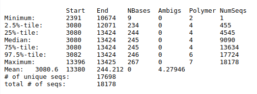
Question
To make sure that everything overlaps the same region we’ll re-run Screen.seqs to get sequences
that start at or before position 3,080 and end at or after position 13,424.
Screen.seqs tool with the following parameters:
Screen.seqsQuestion
Now we know our sequences overlap the same alignment coordinates, we want to make sure they only overlap that region. So we’ll filter the sequences to remove the overhangs at both ends.
In addition, there are many columns in the alignment that only contain external gap characters (i.e. “.”), while columns containing only internal gap characters (i.e., “-“) are not considered. These can be pulled out without losing any information.
Filter.seqs tool with the following parameters:
Screen.seqsThe main questions when analyzing amplicon data are:
The idea is to take the sequences and assign them to a taxon. To do that, we group (or cluster) sequences based on their similarity to defined Operational Taxonomic Units (OTUs): groups of similar sequences that can be treated as a single “genus” or “species” (depending on the clustering threshold).
In 16S metagenomics approaches, OTUs are clusters of similar sequence variants of the 16S rDNA marker gene sequence.
Each of these clusters is intended to represent a taxonomic unit of a bacterial species or genus depending on the sequence similarity threshold.
The first thing we want to do is to further de-noise our sequences from potential sequencing errors,
by pre-clustering the sequences using the Pre.cluster tool, allowing for up to 2 differences between sequences.
Pre.cluster will split the sequences by group and then sort them by abundance,
then go from most abundant to least and identify sequences that differ by no more than 2 nucleotides from on another.
If this is the case, then they get merged.
We generally recommend allowing 1 difference for every 100 basepairs of sequence
Pre.cluster tool with the following parameters:
Filter.seqs runScreen.seqs stepQuestion
We would like to classify the sequences using a training set, which is again is provided on mothur’s MiSeq SOP.
Classify.seqs tool with the following parameters:
Pre.clusterPre.clusterThis step may take a couple of minutes

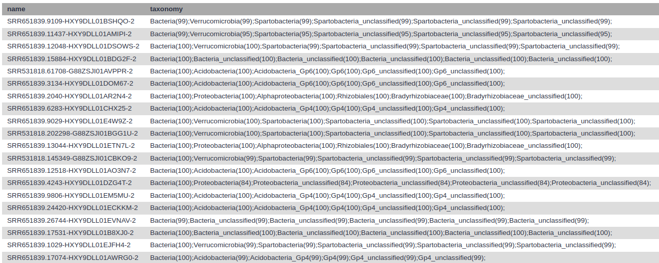 Every read now has a classification.
The next step is to use this information to determine the abundances of the different found taxa:
Cluster.split tool with the following parameters:
Pre.clusterClassify.seqsPre.clusterView the resulting datasets.
We obtain a table with the columns being the different identified OTUs, the rows the different distances and the cells the ids of the sequences identified for these OTUs for the different distances.
Now, we want to know how many sequences are in each OTU from each group with a distance of 0.03 (97% similarity).
Make.shared tool with the following parameters:
Cluster.splitPre.clusterWe want to know the taxonomy for each of our OTUs.
Classify.otu tool with the following parameters:
Cluster.splitPre.clusterClassify.seqsQuestion
We have now determined our OTUs and classified them, but looking at a long text file is not very informative. Let’s visualize our data using Krona:
First we convert our mothur taxonomy file to a format compatible with Krona
Taxonomy-to-Krona tool with the following parameters:
Classify.otu (note: this is a collection input)Krona pie chart tool with the following parameters:
Taxonomy-to-Krona (collection)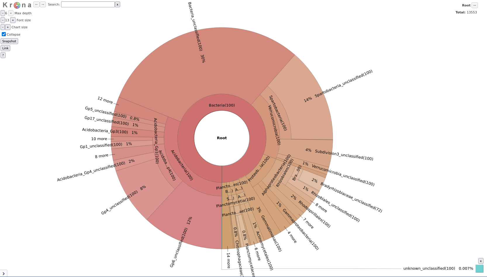
This produced a single plot for both your samples, but what if you want to compare the two samples?
Classify.otu tool
Classify.otu job in your history and see if you can find settings that will give you per-sample taxonomy dataKrona tool
Taxonomy-to-Krona tool with the following parameters:
Classify.otu (note: this is a collection input)Krona pie chart tool with the following parameters:
Taxonomy-to-Krona (collection)In this new Krona output you can switch between the combined plot and the per-sample plots via the selector in the top-left corner.
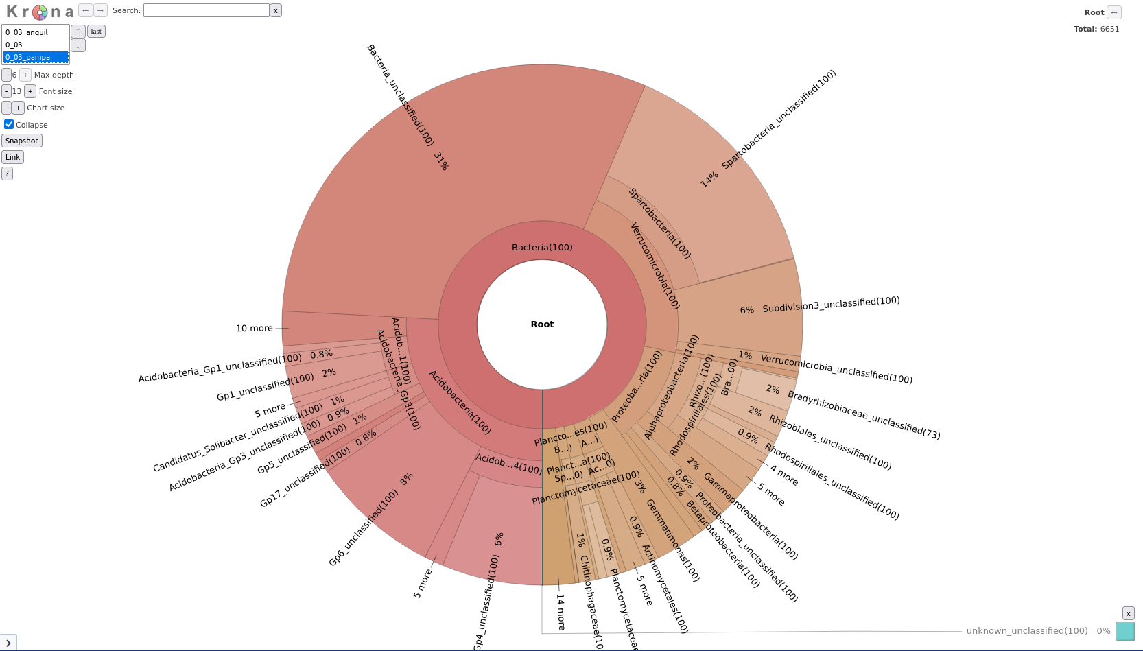
Question
To further explore the community structure, we can visualize it with dedicated tools such as Phinch.
Make.biom tool with the following parameters:
Make.shared outputClassify.otu (collection)name-file.biom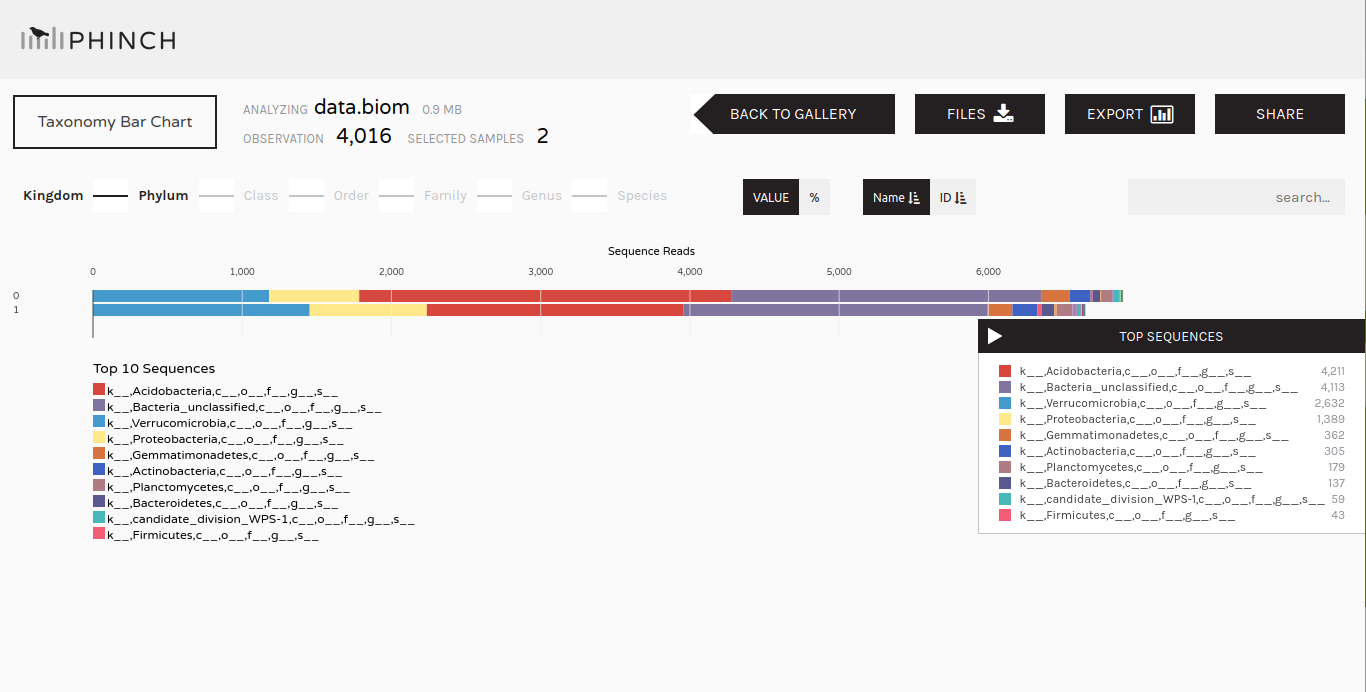
Once we have information about the community structure (OTUs with taxonomic structure), we can do more analysis on it:
In shotgun data, full genomes of the micro-organisms in the environment are sequenced (not only the 16S or 18S).
We can then have access to the rRNA (only a small part of the genomes), but also to the other genes of the micro-organisms.
Using this information, we can try to answer questions such as “What are the micro-organisms doing?” in addition to the question “What micro-organisms are present?”.
https://zenodo.org/record/815875/files/SRR606451_pampa.fasta
As for amplicon data, we can extract taxonomic and community structure information from shotgun data.
Different approaches can be used:
In this tutorial, we use the second approach with MetaPhlAn2. See MetaPhlAn2
This tools is using a database of ~1M unique clade-specific marker genes (not only the rRNA genes) identified from ~17,000 reference (bacterial, archeal, viral and eukaryotic) genomes.
MetaPhlAN2 tool with:
This step may take a couple of minutes.

3 files are generated:
Question
Format MetaPhlAn2 output for Krona tool with:
KRONA pie chart tool with:
Format MetaPhlAn2In the shotgun data, we have access to the gene sequences from the full genome. We use that to identify the genes, associate them with a function, build pathways, etc., to investigate the functional part of the community.
HUMAnN2 tool with:
Import the 3 files whose the name is starting with “humann2”
https://zenodo.org/record/815875/files/humann2_gene_families_abundance.tsv
https://zenodo.org/record/815875/files/humann2_pathways_abundance.tsv
https://zenodo.org/record/815875/files/humann2_pathways_coverage.tsv
HUMAnN2 generates 3 files
A file with the abundance of gene families
Gene family abundance is reported in RPK (reads per kilobase) units to normalize for gene length. It reflects the relative gene (or transcript) copy number in the community.
The “UNMAPPED” value is the total number of reads which remain unmapped after both alignment steps (nucleotide and translated search). Since other gene features in the table are quantified in RPK units, “UNMAPPED” can be interpreted as a single unknown gene of length 1 kilobase recruiting all reads that failed to map to known sequences.
A file with the coverage of pathways
Pathway coverage provides an alternative description of the presence (1) and absence (0) of pathways in a community, independent of their quantitative abundance.
A file with the abundance of pathways
Question
The RPK for the gene families are quite difficult to interpret in term of relative abundance. We decide then to normalize the values
Renormalize a HUMAnN2 generated table tool with:
HUMAnN2Question
