Which species (or genera, families, …) are present in my sample? What are the different approaches and tools to get the community profile of my sample? How can we visualize and compare community profiles?
The investigation of microorganisms present at a specific site and their relative abundance is also called microbial community profiling”. The main objective is to identify the microorganisms that are present within the given sample. This can be achieved for all known microbes, where the DNA sequence specific for a certain species is known.
For that we try to identify the taxon to which each individual read belongs.
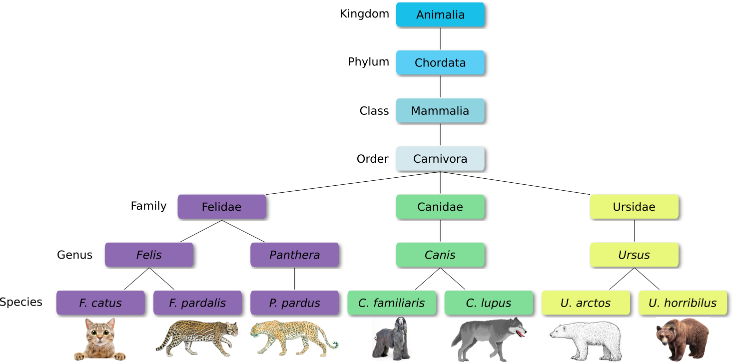
The taxonomic hierarchy includes eight levels: Domain, Kingdom, Phylum, Class, Order, Family, Genus and Species.
Let’s explore taxonomy in the Tree of Life, using Lifemap
For metagenomic data analysis we start with sequences derived from DNA fragments that are isolated from the sample of interest. Ideally, the sequences from all microbes in the sample are present.
The underlying idea of taxonomic assignment is to compare the DNA sequences found in the sample (reads) to DNA sequences of a database. When a read matches a database DNA sequence of a known microbe, we can derive a list with microbes present in the sample.
When talking about taxonomic assignment or taxonomic classification, most of the time we actually talk about two methods, that in practice are often used interchangeably:
The reads can be obtained from amplicon sequencing (e.g. 16S, 18S, ITS), where only specific gene or gene fragments are targeted (using specific primers) or shotgun metagenomic sequencing, where all the accessible DNA of a mixed community is amplified (using random primers).
This tutorial focuses on reads obtained from shotgun metagenomic sequencing.
Tools for taxonomic profiling can be divided into three groups
The comparison of reads to database sequences can be done in different ways, leading to three different types of taxonomic assignment:
Genome based approach
Reads are aligned to reference genomes. Considering the coverage and breadth, genomes are used to measure genome abundance. Furthermore, genes can be analyzed in genomic context. Advantages of this method are the high detection accuracy, that the unclassified percentage is known, that all SNVs can be detected and that high-resolution genomic comparisons are possible. This method takes medium compute cost.
Gene based approach
Reads are aligned to reference genes. Next, marker genes are used to estimate species abundance. Furthermore, genes can be analyzed in isolation for presence or absence in a specific condition. The major advantage is the detection of the pangenome (entire set of genes within a species). Major disadvantages are the high compute cost, low detection accuracy and that the unclassified percentage is unknown. At least intragenic SNVs can be detected and low-resolution genomic comparison is possible.
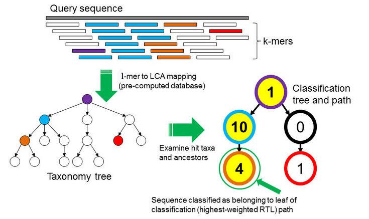
k-mer based approach
Databases as well as the samples DNA are broken into strings of length k
for comparison. From all the genomes in the database, where a specific k-mer is found, a lowest common ancestor (LCA)
tree is derived and the abundance of k-mers within the tree is counted.
This is the basis for a root-to-leaf path calculation, where the path with the highest score is used for classification of the sample.
By counting the abundance of k-mers, also an estimation of relative abundance of taxa is possible.
The major advantage of k-mer based analysis is the low compute cost.
Major disadvantages are the low detection accuracy, that the unclassified percentage is unknown and that there is no gene detection,
no SNVs detection and no genomic comparison possible. An example for a k-mer based analysis tool is Kraken, which will be used in this tutorial
A typical workflow consists of:
FastQC and Trim Galore! or Cutadapt) and (optionally) dereplication (VSearch)Kraken2 or MetaPhlAn2) and visualization (KRONA, GraPhlAn)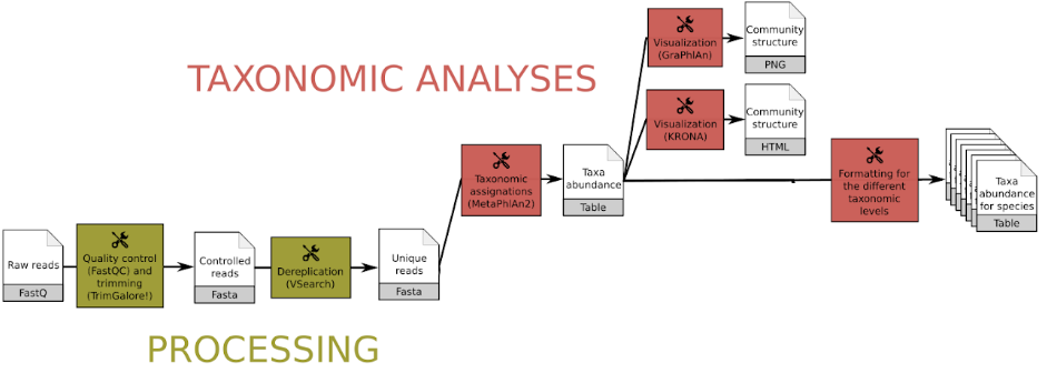
The dataset we will use for this tutorial comes from an oasis in the Mexican desert called Cuatro Ciénegas.
The researchers were interested in genomic traits that affect the rates and costs of biochemical information processing within cells. They performed a whole-ecosystem experiment, thus fertilizing the pond to achieve nutrient enriched conditions.
Here we will use 2 datasets:
The reads have been trimmed using cutadapt as explained in the Quality control tutorial.
NOTE! Please, use:
https://zenodo.org/record/7871630/files/JC1A_R1.fastqsanger.gz
https://zenodo.org/record/7871630/files/JC1A_R2.fastqsanger.gz
https://zenodo.org/record/7871630/files/JP4D_R1.fastqsanger.gz
https://zenodo.org/record/7871630/files/JP4D_R2.fastqsanger.gz
To find out which microorganisms are present, we will compare the reads of the sample to a reference database, i.e. sequences of known microorganisms stored in a database, using Kraken2
In the k-mer approach for taxonomy classification, we use a database containing DNA sequences of genomes whose taxonomy we already know. On a computer, the genome sequences are broken into short pieces of length k (called k-mers), usually 30bp.
Kraken2:
For this tutorial, we will use the PlusPF database which contains the Standard (archaea, bacteria, viral, plasmid, human, UniVec_Core), protozoa and fungi data.
Kraken2 Tool with the following parameters:
A confidence score of 0.1 means that at least 10% of the k-mers should match entries in the database. This value can be reduced if a less restrictive taxonomic assignation is desired.
Kraken2 will create two outputs for each dataset: Classification and Report
C/U: a one letter indicating if the sequence classified or unclassifiedread1|read2 for paired reads)For example, 562:13 561:4 A:31 0:1 562:3 would indicate that:
|:| indicates end of first read, start of second read for paired reads
For JC1A:
C1  C2                                                      C3      C4      C5
U   MISEQ-LAB244-W7:91:000000000-A5C7L:1:1101:13417:1998    0       151|190 A:18 0:14 2055:5 0:1 2220095:5 0:74 |:| 0:3 A:54 2:1 0:32 204455:1 2823043:5 0:60
U   MISEQ-LAB244-W7:91:000000000-A5C7L:1:1101:15782:2187    0       169|173 0:101 37329:1 0:33 |:| 0:10 2751189:5 0:30 1883:2 0:39 2609255:5 0:48
U   MISEQ-LAB244-W7:91:000000000-A5C7L:1:1101:11745:2196    0       235|214 0:173 2282523:5 2746321:2 0:21 |:| 0:65 2746321:2 2282523:5 0:108
U   MISEQ-LAB244-W7:91:000000000-A5C7L:1:1101:18358:2213    0       251|251 0:35 281093:5 0:3 651822:5 0:145 106591:3 0:21 |:| 0:64 106591:3 0:145 651822:5
U   MISEQ-LAB244-W7:91:000000000-A5C7L:1:1101:14892:2226    0       68|59   0:34 |:| 0:25
U   MISEQ-LAB244-W7:91:000000000-A5C7L:1:1101:18764:2247    0       146|146 0:112 |:| 0:112
C   MISEQ-LAB244-W7:91:000000000-A5C7L:1:1101:12147:2252    9606    220|220 9606:148 0:19 9606:19 |:| 9606:19 0:19 9606:148
U   MISEQ-LAB244-W7:91:000000000-A5C7L:1:1101:14052:2291    0       118|85  0:84 |:| 0:7 5679:5 0:39
C   MISEQ-LAB244-W7:91:000000000-A5C7L:1:1101:18387:2294    9606    241|241 9606:207 |:| 9606:207
U   MISEQ-LAB244-W7:91:000000000-A5C7L:1:1101:13378:2301    0       164|98  0:130 |:| 0:64
Question For JC1A sample:
Column 1    Column 2    Column 3    Column 4    Column 5    Column 6
76.86 	    105399      105399      U 	        0           unclassified
23.14 	    31740       1197 	    R 	        1           root
22.20 	    30448       312 	    R1 	        131567      cellular organisms
12.58 	    17254       3767 	    D 	        2           Bacteria
8.77 	    12027       2867 	    P 	        1224        Proteobacteria
4.94 	    6779        3494 	    C 	        28211       Alphaproteobacteria
1.30 	    1782        1085 	    O 	        204455      Rhodobacterales
0.43 	    593         461 	    F 	        31989       Rhodobacteraceae
0.05 	    74          53          G 	        265         Paracoccus
0.01 	    10          10          S 	        82367       Paracoccus pantotrophus
0.00 	    6           6           S 	        1545044     Paracoccus sanguinis
0.00 	    5           0           G1 	        2688777     unclassified Paracoccus
0.00 	    4           4           S 	        2589076     Paracoccus sp. AK26
0.00 	    1           1           S 	        2895796     Paracoccus sp. MA
0.01 	    17          16          G 	        1060        Rhodobacter
0.00 	    1           0           G1 	        196779      unclassified Rhodobacter
0.00 	    1           1           S 	        2033869     Rhodobacter sp. CZR27
0.01 	    17          15          G 	        34008       Rhodovulum
0.00 	    2           0           G1 	        2631432     unclassified Rhodovulum
0.00 	    2           2           S 	        1564506     Rhodovulum sp. P5
Taxa that are not at any of these 10 ranks have a rank code that is formed by using the rank code of the closest ancestor rank with a number indicating the distance from that rank.
E.g., G2 is a rank code indicating a taxon is between genus and species and the grandparent taxon is at the genus rank.
Question
Getting an overview of the assignation is not straightforward with the Kraken2 outputs directly.
We can use visualisation tools for that.
A simple and worthwile addition to Kraken for better abundance estimates is called Bracken
(Bayesian Reestimation of Abundance after Classification with Kraken).
Instead of only using proportions of classified reads, it takes a probabilistic approach to generate final abundance profiles. It works by re-distributing reads in the taxonomic tree: Reads assigned to nodes above the species level are distributed down to the species nodes, while reads assigned at the strain level are re-distributed upward to their parent species
Estimate Abundance at Taxonomic Level Tool with the following parameters:
NOTE! It is important to choose the same database that you also chose for Kraken2
Bracken output file format (tabular):
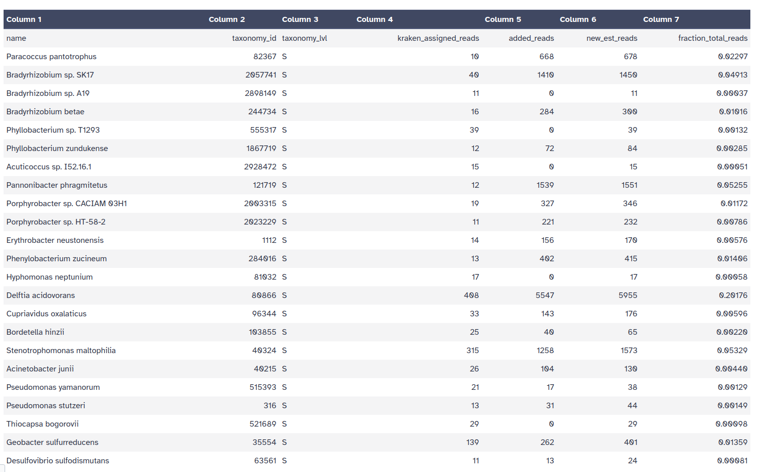
Kraken style report
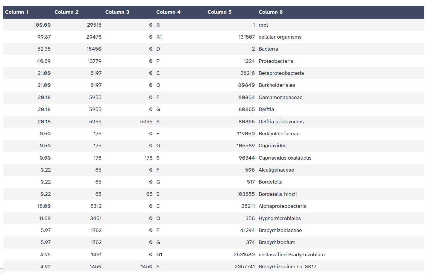
Getting an overview of the assignation is not straightforward with the Kraken2 outputs directly. Once we have assigned the corresponding taxa to each sequence, the next step is to properly visualize the data. There are several tools for that:
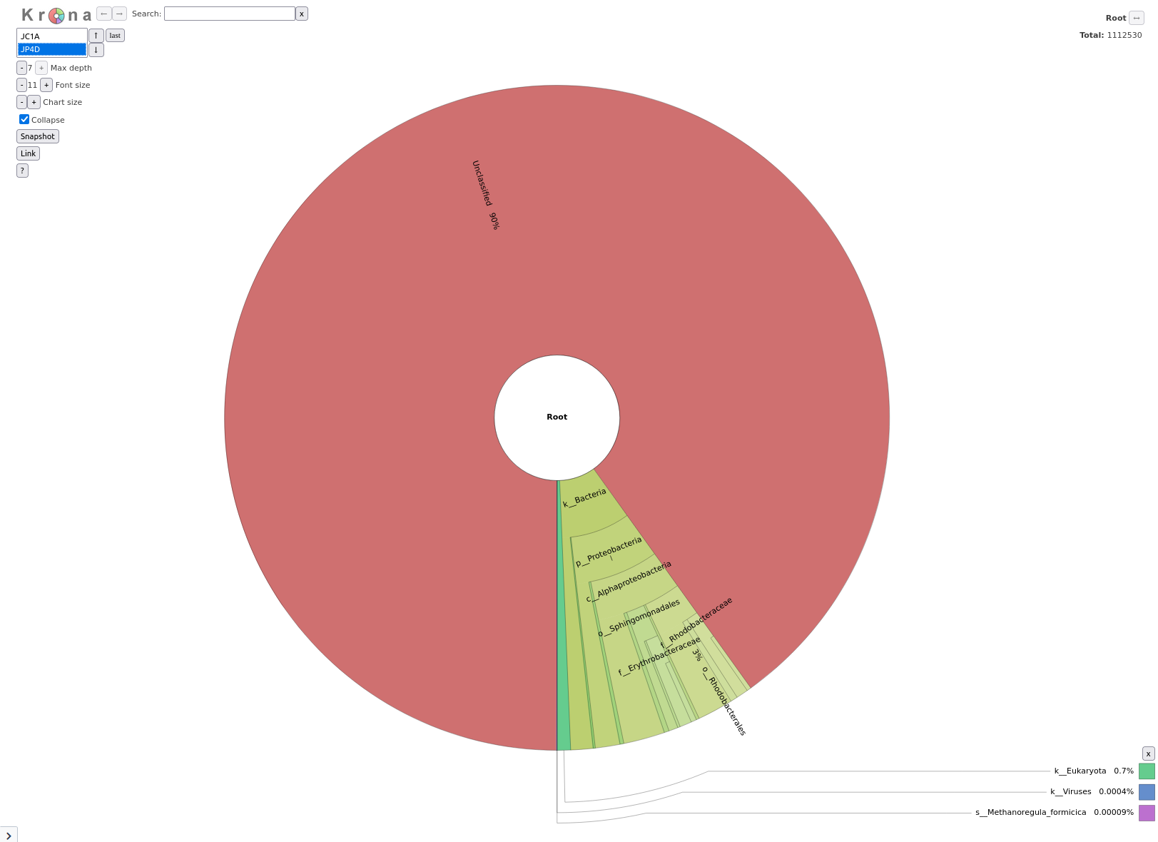
Krona creates an interactive HTML file allowing hierarchical data to be explored with zooming, multi-layered pie charts.
With this tool, we can easily visualize the composition of the bacterial communities and compare how the populations of microorganisms are modified according to the conditions of the environment.
Kraken outputs can not be given directly to Krona, they first need to be converted.
Krakentools is a suite of tools to work on Kraken outputs.
It include a tool designed to translate results of the Kraken metagenomic classifier
to the full representation of NCBI taxonomy.
The output of this tool can be directly visualized by the Krona tool.
Krakentools: Convert kraken report file Tool with the following parameters:
Kraken105399 Unclassified
3868 k__Bacteria
2867 k__Bacteria p__Proteobacteria
3494 k__Bacteria p__Proteobacteria c__Alphaproteobacteria
1085 k__Bacteria p__Proteobacteria c__Alphaproteobacteria o__Rhodobacterales
461 k__Bacteria p__Proteobacteria c__Alphaproteobacteria o__Rhodobacterales f__Rhodobacteraceae
53 k__Bacteria p__Proteobacteria c__Alphaproteobacteria o__Rhodobacterales f__Rhodobacteraceae g__Paracoccus
10 k__Bacteria p__Proteobacteria c__Alphaproteobacteria o__Rhodobacterales f__Rhodobacteraceae g__Paracoccus s__Paracoccus_pantotrophus
6 k__Bacteria p__Proteobacteria c__Alphaproteobacteria o__Rhodobacterales f__Rhodobacteraceae g__Paracoccus s__Paracoccus_sanguinis
4 k__Bacteria p__Proteobacteria c__Alphaproteobacteria o__Rhodobacterales f__Rhodobacteraceae g__Paracoccus s__Paracoccus_sp._AK26
Question
Let’s now run Krona
Krona pie chart Tool with the following parameters:
Krakentools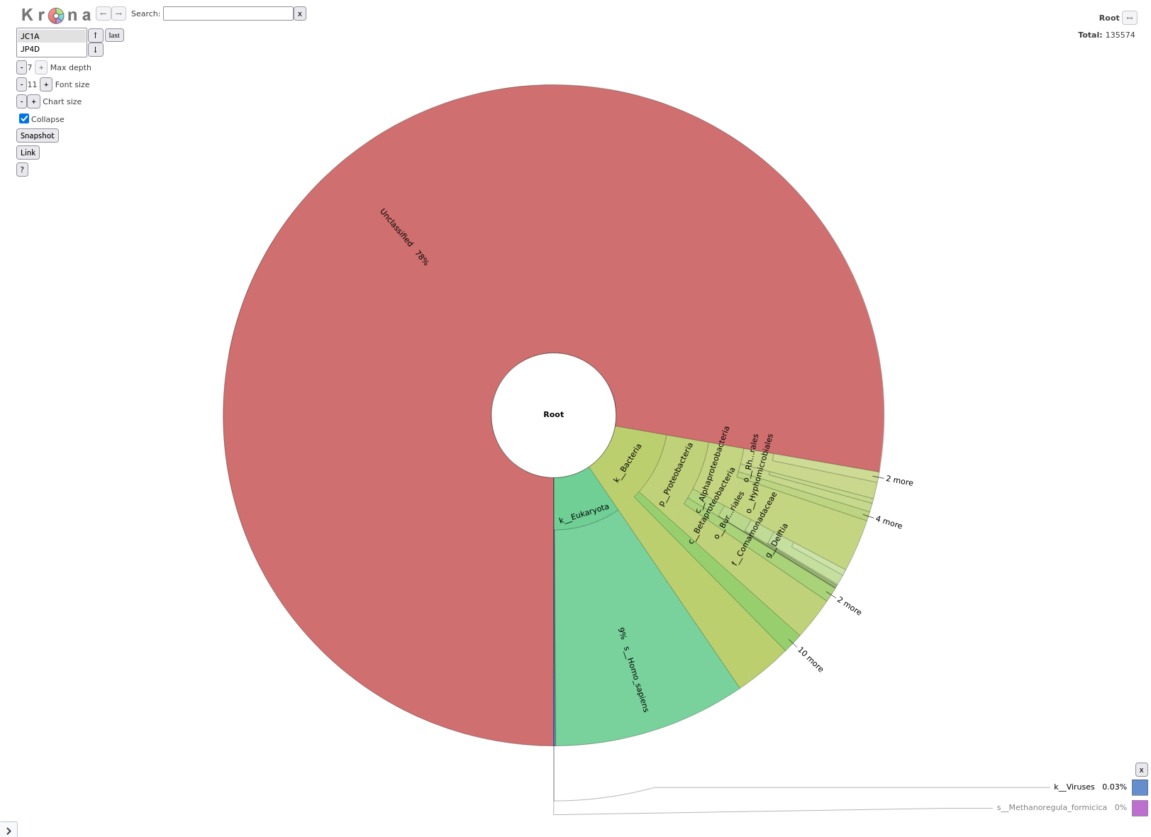
Question
Phinch is another tools to visualize large biological datasets like our taxonomic classification
As a first step, we need to convert the Kraken output file into a kraken-biom file to make it accessible for Phinch.
For this, we need to add a metadata file. When generating a metadata file for your own data, you can take this as an example and apply the general guidelines:
#SampleID, and the data in this column must contain unique (short and meaningful) sample identifiers containing only alphanumeric and period (.) characters.BarcodeSequence, where each value in that column corresponds to the barcode used for each sampleSmoker column would include either Yes or No. Note that the data in each column is assumed to be categorical unless specified otherwise. Categorical data columns must include at least 2 unique values per column. All metadata must be composed of:
_),.),-),+),%), ),;),:),,),/) characters.NA; do not leave blanks.Description. Information in this column includes information that is unique to each sample, such as the medications taken by the patient, or any other descriptive information. The same character restrictions that apply to the metadata columns in guideline four apply to sample descriptions. Sample/Run Description should be kept brief, if possible.# character, immediately following the header line (See example format below.)#) throughout the metadata, with the exception of any additional run description lines that immediately follow the initial header line.
#SampleID BarcodeSequence LinkerPrimerSequence Treatment DOB Description
#Example mapping file for the QIIME analysis package.
#These 9 samples are from a study of the effects of
#exercise and diet on mouse cardiac physiology (Crawford, et al, PNAS, 2009).
PC.354 AGCACGAGCCTA YATGCTGCCTCCCGTAGGAGT Control 20061218 Control_mouse__I.D._354
PC.355 AACTCGTCGATG YATGCTGCCTCCCGTAGGAGT Control 20061218 Control_mouse__I.D._355
PC.356 ACAGACCACTCA YATGCTGCCTCCCGTAGGAGT Control 20061126 Control_mouse__I.D._356
PC.481 ACCAGCGACTAG YATGCTGCCTCCCGTAGGAGT Control 20070314 Control_mouse__I.D._481
PC.593 AGCAGCACTTGT YATGCTGCCTCCCGTAGGAGT Control 20071210 Control_mouse__I.D._593
PC.607 AACTGTGCGTAC YATGCTGCCTCCCGTAGGAGT Fast 20071112 Fasting_mouse__I.D._607
PC.634 ACAGAGTCGGCT YATGCTGCCTCCCGTAGGAGT Fast 20080116 Fasting_mouse__I.D._634
PC.635 ACCGCAGAGTCA YATGCTGCCTCCCGTAGGAGT Fast 20080116 Fasting_mouse__I.D._635
PC.636 ACGGTGAGTGTC YATGCTGCCTCCCGTAGGAGT Fast 20080116 Fasting_mouse__I.D._636
https://zenodo.org/record/7871630/files/metadata.tabular
Kraken-biom Tool (to convert Kraken2 report into the correct format for Phinch) with the following parameters:
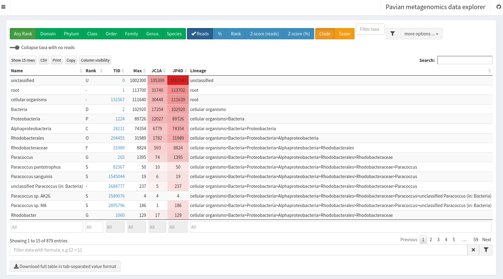
Proceed to gallery to see an overview of all visualization optionsPavian (pathogen visualization and more) is an interactive visualization tool for metagenomic data. It was developed for the clinical metagenomic problem to find a disease-causing pathogen in a patient sample, but it is useful to analyze and visualize any kind of metagenomics data.
KrakenSave table
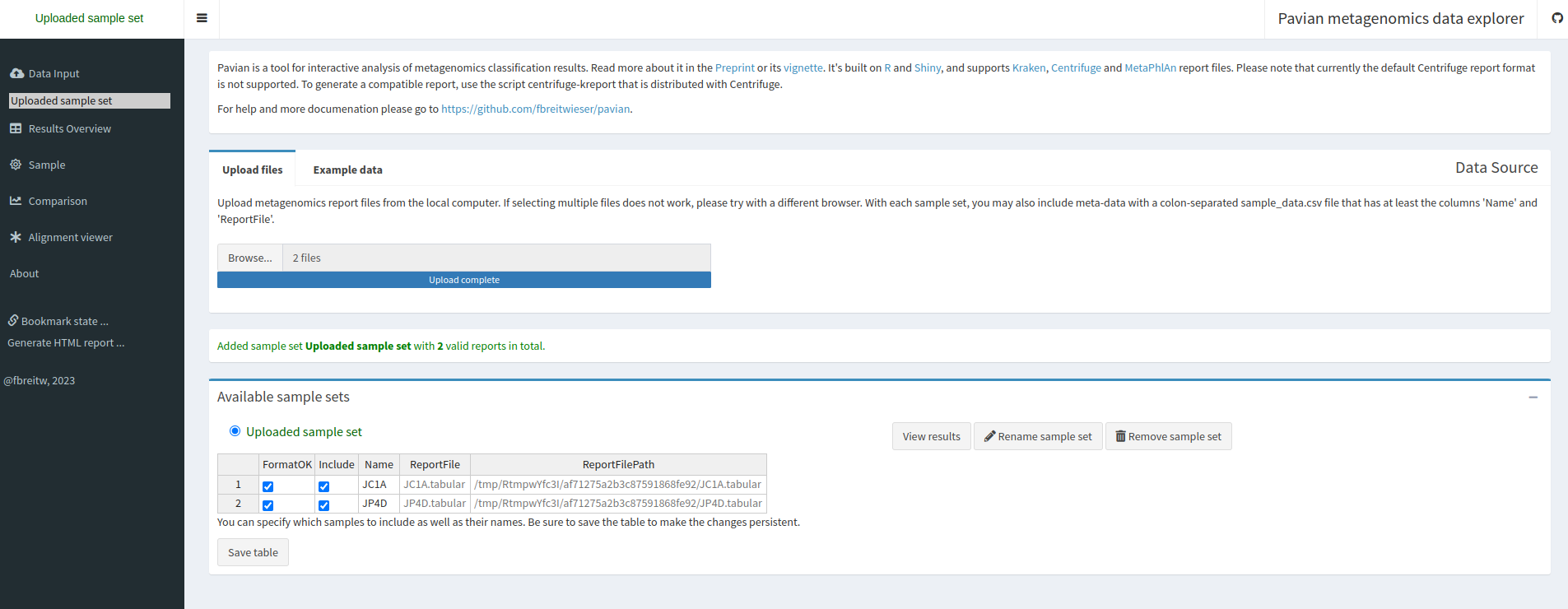
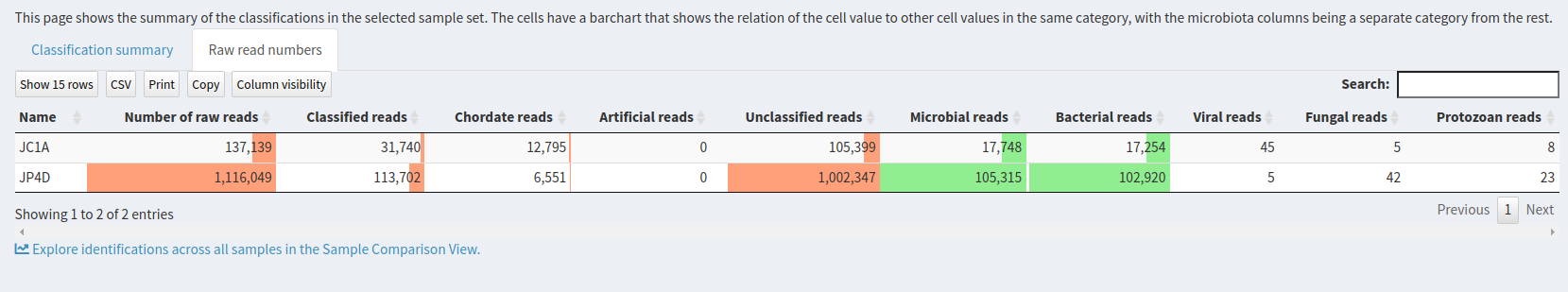
Result Overview.
This page shows the summary of the classifications in the selected sample set: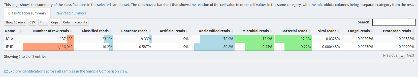
Question
Let’s now inspect assignements to reads per sample.
Sample in the left panelJC1A in the Select sample drop-down on the topThe first view gives a Sankey diagram for one sample:
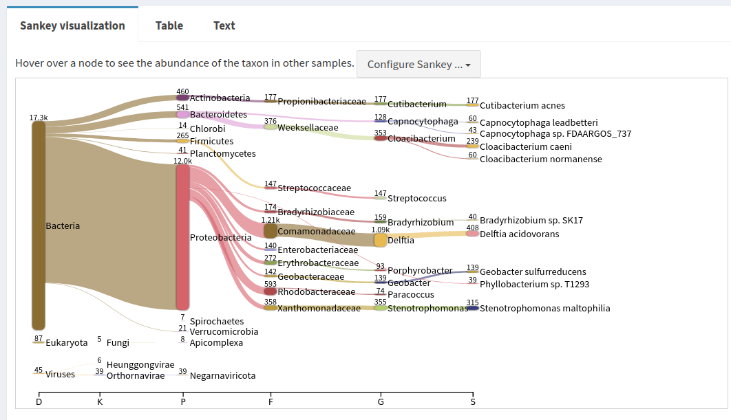
Proteobacteria in the Sankey plot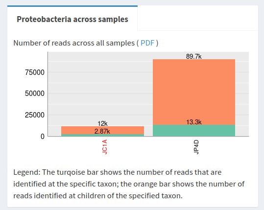
Question
Comparison in the left panel% and unclick Reads in the blue area drop-down on the topDomain green button
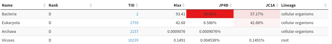
Homo sapiens in the Filter taxa box below the green buttons
Class green button
MetaPhlAn is a computational tool for profiling the composition of microbial communities (Bacteria, Archaea and Eukaryotes) from metagenomic shotgun sequencing data (i.e. not 16S) at species-level.
It allows:
The basic usage of MetaPhlAn consists in the identification of the clades (from phyla to species and strains in particular cases) present in the microbiota obtained from a microbiome sample and their relative abundance.
MetaPhlAn in Galaxy can not directly take as input a paired collection but expect 2 collections:
1 with forward data and 1 with reverse.
Before launching MetaPhlAn, we need to split our input paired collection.
Unzip collection Tool with the following parameters:
MetaPhlAn Tool with the following parameters:
Unzip collection with forward in the nameUnzip collection with reveerse in the name5 files and a collection are generated by MetaPhlAn:
Predicted taxon relative abundances: tabular files with the community profile
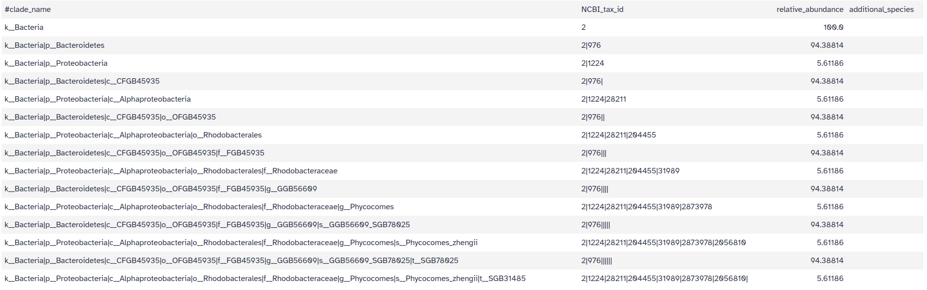 Each line contains 4 columns:
k__) to more precise taxaQuestion
MetaPhlAn, compared to the one identified with Kraken !!Predicted taxon relative abundances for Krona: same information as the previous files but formatted for > visualization using Krona
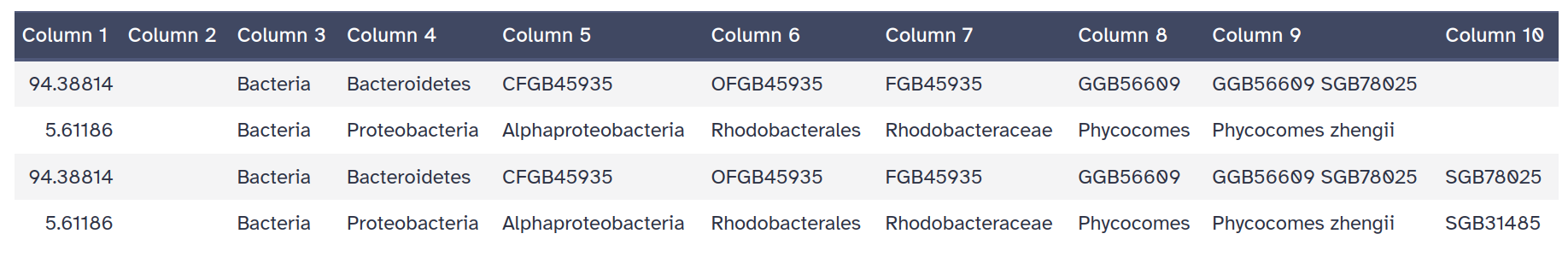
Each line represent an identified taxons with 9 columns:
BIOM file with community profile in BIOM format
Bowtie2 output and SAM file with the results of the sequence mapping on the reference databaseLet’s now run Krona to visualize the communities
Krona pie chart Tool with the following parameters:
Metaphlan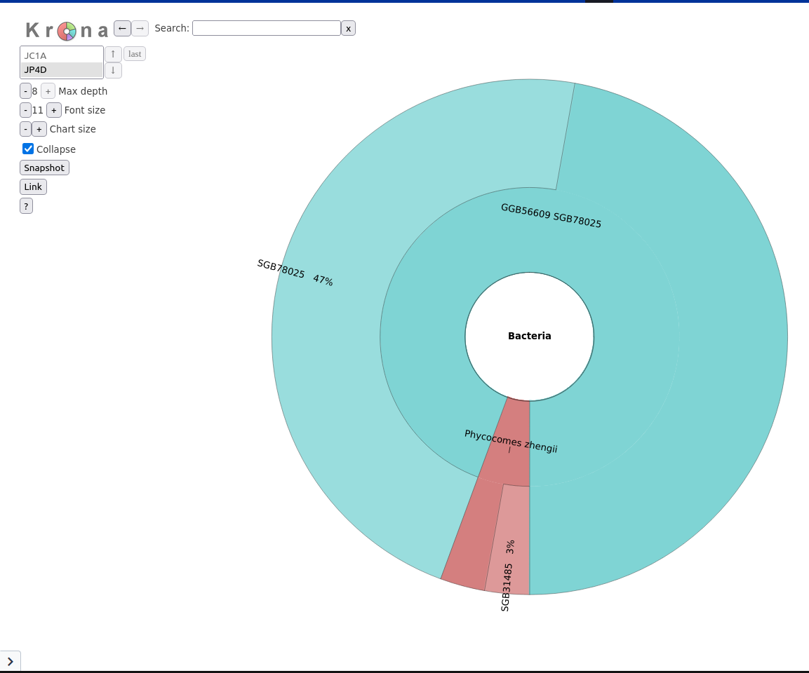
The community looks a lot less diverse than with Kraken.
However, Kraken is also known to have high number of false positive. A benchmark dataset or mock community where the community DNA content is known would be required to correctly judge which tool provides the better taxonomic classification.
GraPhlAn is another software tool for producing high-quality circular representations of taxonomic and phylogenetic trees.
We first need to convert the MetaPhlAn output using Export to GraPhlAn.
This conversion software tool produces both annotation and tree file for GraPhlAn.
Export to GraPhlAn need the MetaPhlAn table with predicted taxon abundance with only 2 columns: the lineage and the abundance.
Cut Tool with the following parameters:
MetaPhlAn)Export to GraPhlAn Tool with the following parameters:
Generation, personalization and annotation of tree Tool with the following parameters:
Export to GraPhlAn)Export to GraPhlAn)GraPhlAn Tool with the following parameters:
GraPhlAn output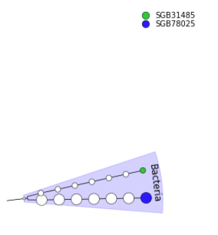
In this tutorial, we look how to get the community profile from microbiome data.
Kraken or MetaPhlAn can be used in Galaxy for taxonomic assignment
Krona, Pavian or GraPhlAnNow, it’s your turn!