16S Microbial Analysis with Mothur

What is the effect of normal variation in the gut microbiome on host health?

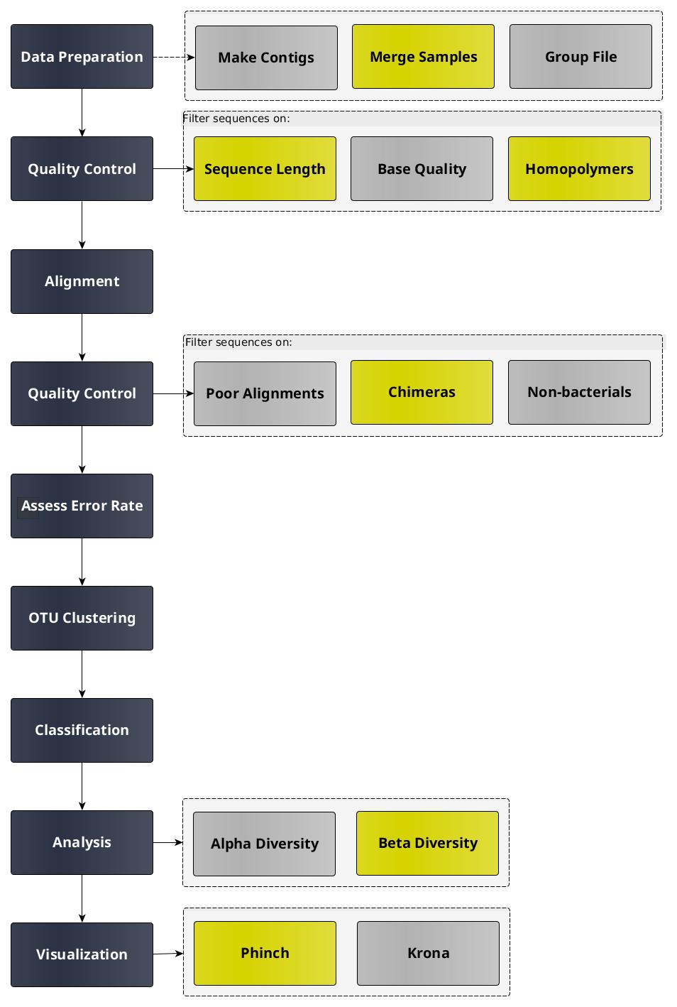
In this tutorial we will perform an analysis based on the Standard Operating Procedure (SOP) for MiSeq data, developed by the Schloss lab, the creators of the mothur software package.

NOTE: In this tutorial we use 16S rRNA data, but similar pipelines can be used for WGS data.

Obtaining and preparing data

In this tutorial we use the dataset generated by the Schloss lab to illustrate their MiSeq SOP.

They describe the experiment as follows:

“The Schloss lab is interested in understanding the effect of normal variation in the gut microbiome on host health. To that end, we collected fresh feces from mice on a daily basis for 365 days post weaning. During the first 150 days post weaning (dpw), nothing was done to our mice except allow them to eat, get fat, and be merry.

We were curious whether the rapid change in weight observed during the first 10 dpw affected the stability microbiome compared to the microbiome observed between days 140 and 150.”

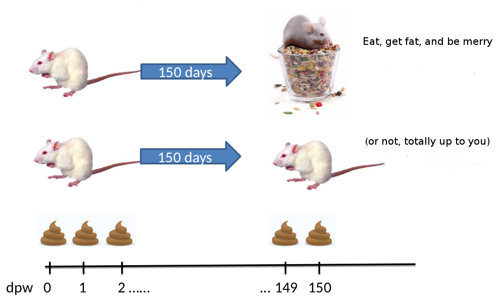
To speed up analysis for this tutorial, we will use only a subset of this data. We will look at a single mouse at 10 different time points (5 early, 5 late).

In order to assess the error rate of the analysis pipeline and experimental setup, the Schloss lab additionally sequenced a mock community with a known composition (genomic DNA from 21 bacterial strains). The sequences used for this mock sample are contained in the file HMP_MOCK.v35.fasta

Go Up

Importing the data into Galaxy

For this tutorial, you are given 10 pairs of files. For example, the following pair of files:

F3D0_S188_L001_R1_001.fastq
F3D0_S188_L001_R2_001.fastq

The first part of the file name indicates the sample; F3D0 here signifies that this sample was obtained from Female 3 on Day 0. The rest of the file name is identical, except for _R1 and _R2, this is used to indicate the forward and reverse reads respectively.

1. Create a new history
2. Upload datasets

   https://zenodo.org/record/800651/files/F3D0_R1.fastq
   https://zenodo.org/record/800651/files/F3D0_R2.fastq
   https://zenodo.org/record/800651/files/F3D141_R1.fastq
   https://zenodo.org/record/800651/files/F3D141_R2.fastq
   https://zenodo.org/record/800651/files/F3D142_R1.fastq
   https://zenodo.org/record/800651/files/F3D142_R2.fastq
   https://zenodo.org/record/800651/files/F3D143_R1.fastq
   https://zenodo.org/record/800651/files/F3D143_R2.fastq
   https://zenodo.org/record/800651/files/F3D144_R1.fastq
   https://zenodo.org/record/800651/files/F3D144_R2.fastq
   https://zenodo.org/record/800651/files/F3D145_R1.fastq
   https://zenodo.org/record/800651/files/F3D145_R2.fastq
   https://zenodo.org/record/800651/files/F3D146_R1.fastq
   https://zenodo.org/record/800651/files/F3D146_R2.fastq
   https://zenodo.org/record/800651/files/F3D147_R1.fastq
   https://zenodo.org/record/800651/files/F3D147_R2.fastq
   https://zenodo.org/record/800651/files/F3D148_R1.fastq
   https://zenodo.org/record/800651/files/F3D148_R2.fastq
   https://zenodo.org/record/800651/files/F3D149_R1.fastq
   https://zenodo.org/record/800651/files/F3D149_R2.fastq
   https://zenodo.org/record/800651/files/F3D150_R1.fastq
   https://zenodo.org/record/800651/files/F3D150_R2.fastq
   https://zenodo.org/record/800651/files/F3D1_R1.fastq
   https://zenodo.org/record/800651/files/F3D1_R2.fastq
   https://zenodo.org/record/800651/files/F3D2_R1.fastq
   https://zenodo.org/record/800651/files/F3D2_R2.fastq
   https://zenodo.org/record/800651/files/F3D3_R1.fastq
   https://zenodo.org/record/800651/files/F3D3_R2.fastq
   https://zenodo.org/record/800651/files/F3D5_R1.fastq
   https://zenodo.org/record/800651/files/F3D5_R2.fastq
   https://zenodo.org/record/800651/files/F3D6_R1.fastq
   https://zenodo.org/record/800651/files/F3D6_R2.fastq
   https://zenodo.org/record/800651/files/F3D7_R1.fastq
   https://zenodo.org/record/800651/files/F3D7_R2.fastq
   https://zenodo.org/record/800651/files/F3D8_R1.fastq
   https://zenodo.org/record/800651/files/F3D8_R2.fastq
   https://zenodo.org/record/800651/files/F3D9_R1.fastq
   https://zenodo.org/record/800651/files/F3D9_R2.fastq
   https://zenodo.org/record/800651/files/Mock_R1.fastq
   https://zenodo.org/record/800651/files/Mock_R2.fastq
   

3. Import Reference Data

   https://zenodo.org/record/800651/files/HMP_MOCK.v35.fasta
   https://zenodo.org/record/800651/files/silva.v4.fasta
   https://zenodo.org/record/800651/files/trainset9_032012.pds.fasta
   https://zenodo.org/record/800651/files/trainset9_032012.pds.tax
   https://zenodo.org/record/800651/files/mouse.dpw.metadata
   

Go Up

Organizing our data into a paired collection

Now that’s a lot of files to manage. Luckily Galaxy can make life a bit easier by allowing us to create dataset collections. This enables us to easily run tools on multiple datasets at once.

Since we have paired-end data, each sample consist of two separate fastq files, one containing the forward reads, and one containing the reverse reads.

We can recognize the pairing from the file names, which will differ only by _R1 or _R2 in the filename. We can tell Galaxy about this paired naming convention, so that our tools will know which files belong together. We do this by building a List of Dataset Pairs

1. Click on the checkmark icon param-check at top of your history.
2. Select all the FASTQ files (40 in total)
   • type fastq in the search bar at the top of your history to filter only the FASTQ files; you can now use the All button at the top instead of having to individually select all 40 input files.
   • Click on All 40 selected
   • Select Build List of Dataset Pairs from the dropdown menu

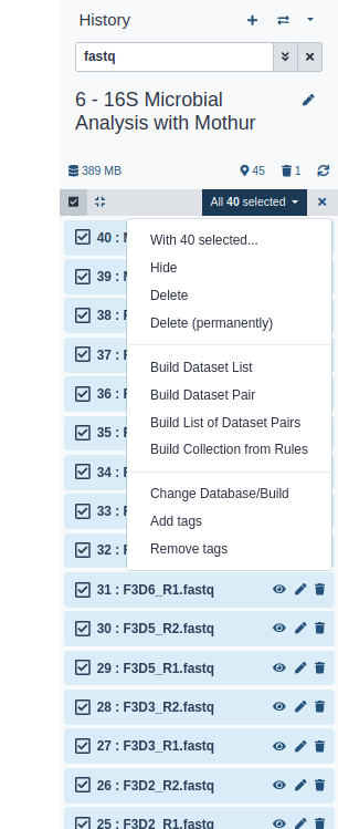
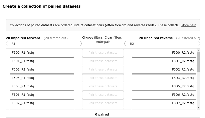
   In the next dialog window you can create the list of pairs. By default Galaxy will look for pairs of files that differ only by a _1 and _2 part in their names. In our case however, these should be _R1 and _R2.

3. Click on “Choose Filters” and select Forward: _R1, Reverse: _R2 (note that you can also enter Filters manually in the text fields on the top) You should now see a list of pairs suggested by Galaxy:
4. Click on Auto-pair to create the suggested pairs.
5. Name the pairs
6. Name your collection at the bottom right of the screen
7. Click the Create Collection button.

Go Up

Quality Control

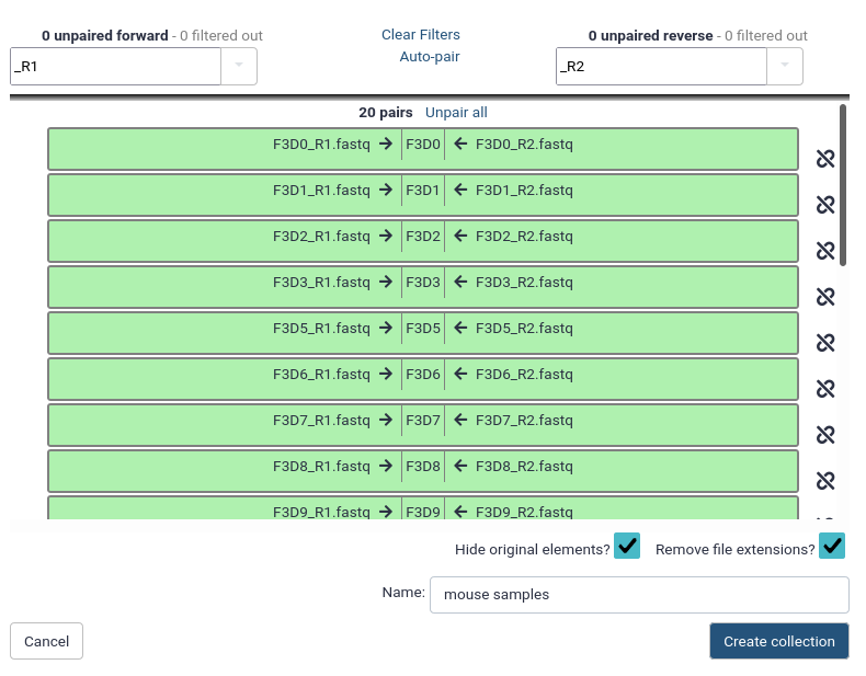
Before starting any analysis, it is always a good idea to assess the quality of your input data and improve it where possible by trimming and filtering reads.

The mothur toolsuite contains several tools to assist with this task.

1. Merging our reads into contigs
2. Filtering and trimming of reads based on quality score and several other metrics.

Go Up

Create contigs from paired-end reads

In this experiment, paired-end sequencing of the ~253 bp V4 region of the 16S rRNA gene was performed. The sequencing was done from either end of each fragment. Because the reads are about 250 bp in length, this results in a significant overlap between the forward and reverse reads in each pair. We will combine these pairs of reads into contigs.

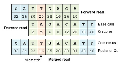
The Make.contigs tool creates the contigs, and uses the paired collection as input:

1. will look at each pair
2. take the reverse complement reverse read
3. determine the overlap between the two sequences.

Where an overlapping base call differs between the two reads, the quality score is used to determine the consensus base call.

A new quality score is derived by combining the two original quality scores in both of the reads for all the overlapping positions.`

Go Up

Combine forward and reverse reads into contigs

1. Make.contigs Tool with the following parameters:
   • Way to provide files: Multiple pairs - Combo mode
   • Fastq pairs: the collection you just created
   • Leave all other parameters to the default settings

This step combined the forward and reverse reads for each sample, and also combined the resulting contigs from all samples into a single file.

So we have gone from a paired collection of 20x2 FASTQ files, to a single FASTA file.

In order to retain information about which reads originated from which samples, the tool also output a group file. View that file now, it should look something like this:

Go Up

Data Cleaning

As the next step, we want to improve the quality of our data. But first, let’s get a feel of our dataset:

Summarize data

1. Summary.seqs Tool with the following parameters:
   • fasta: the trim.contigs.fasta file created by Make.contigs tool
   • Output logfile?: yes

The summary output files give information per read. The logfile outputs also contain some summary statistics:

            Start   End	        NBases      Ambigs      Polymer     NumSeqs
Minimum:    1	    248	        248         0	        3           1
2.5%-tile:  1	    252	        252         0	        3           3810
25%-tile:   1	    252	        252         0	        4           38091
Median:     1	    252	        252         0	        4           76181
75%-tile:   1	    253	        253         0	        5           114271
97.5%-tile: 1	    253	        253         6	        6           148552
Maximum:    1	    502	        502         249	        243         152360
Mean:       1	    252.811	252.811	    0.70063     4.44854
# of Seqs:	152360

In this dataset:

• Almost all of the reads are between 248 and 253 bases long.
• 2,5% or more of our reads had ambiguous base calls (Ambigs column).
• The longest read in the dataset is 502 bases.
• There are 152,360 sequences.

Our region of interest, the V4 region of the 16S gene, is only around 250 bases long. Any reads significantly longer than this expected value likely did not assemble well in the Make.contigs step.

Furthermore, we see that 2,5% of our reads had between 6 and 249 ambiguous base calls (Ambigs column). In the next steps we will clean up our data by removing these problematic reads.

We do this data cleaning using the Screen.seqs tool, which removes:

• sequences with ambiguous bases (maxambig) and
• contigs longer than a given threshold (maxlength).

Go Up

Filter reads based on quality and length

1. Screen.seqs Tool with the following parameters
   • fasta: the trim.contigs.fasta file created by Make.contigs tool
   • group: the group file created in the Make.contigs tool step
   • maxlength: 275
   • maxambig: 0

Question How many reads were removed in this screening step?

Go Up

Optimize files for computation

Because we are sequencing many of the same organisms, we anticipate that many of our sequences are duplicates of each other.

Remove duplicate sequences

1. Unique.seqs tool with the following parameters:
   • fasta: the good.fasta file from Screen.seqs
   • output format: Name File

2. View the resulting datasets.

   Unique.seqs tool outputs two files:

   1. a fasta file containing only the unique sequences
   2. a names file consisting of two columns:
      • the first contains the sequence names for each of the unique sequences,
      • the second column contains all other sequence names that are identical to the representative sequence in the first column.

Question

1. How many sequences were unique?
2. How many duplicates were removed?

Here we see that this step has greatly reduced the size of our sequence file; not only will this speed up further computational steps, it will also greatly reduce the amount of disk space (and your Galaxy quota) needed to store all the intermediate files generated during this analysis.

To recap, we now have the following files:

• a FASTA file containing every distinct sequence in our dataset (the representative sequences) from Unique.seqs
• a names file containing the list of duplicate sequences (from Unique.seqs)
• a group file containing information about the samples each read originated from (from Screen.seqs)

To further reduce file sizes and streamline analysis, we can use the Count.seqs tool to combine the group file and the names file into a single count table.

Go Up

Generate count table

1. Count.seqs tool with the following parameters:
   • name: the name file from Unique.seqs
   • Use a group file: yes
   • group: the group file from Screen.seqs

2. View the resulting datasets.

   The first column contains the read names of the representative sequences, and the subsequent columns contain the number of duplicates of this sequence observed in each sample.

Go Up

Sequence Alignment

We are now ready to align our sequences to the reference alignment. This is an important step to improve the clustering of your OTUs.

In mothur this is done by determining for each unique sequence the entry of the reference database that has the most k-mers in common (i.e. the most substring of fixed length k).

For the reference sequence with the most common k-mers and the unique sequence a standard global sequence alignment is computed (using the Needleman-Wunsch algorithm).

Go Up

Align sequences

1. Align.seqs Tool with the following parameters:
   • fasta: the fasta output from Unique.seqs tool
   • reference: silva.v4.fasta reference file from your history
2. View the resulting datasets.

At first glance, it might look like there is not much information there. We see our read names, but only period . characters below it.

>2_F3D0
............................................................................
>3_F3D0
............................................................................
>4_F3D0
............................................................................

This is because the V4 region is located further down our reference database and nothing aligns to the start of it.

If you scroll to right you will start seeing some more informative bits:

.....T-------AC---GG-AG-GAT------------

Here we start seeing how our sequences align to the reference database. There are different alignment characters in this output:

• .: terminal gap character (before the first or after the last base in our query sequence)
• -: gap character within the query sequence

We will cut out only the V4 region in a later step (Filter.seqs tool)

Go Up

Summarize the quality of alignment

1. Summary.seqs Tool with the following parameters:

   • fasta: the align output from Align.seqs tool
   • count: count_table output from Count.seqs tool
   • Output logfile?: yes

2. View the log output.

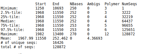
The Start and End columns tell us that the majority of reads aligned between positions 1968 and 11550, which is what we expect to find given the reference file we used.

However, some reads align to very different positions, which could indicate insertions or deletions at the terminal ends of the alignments or other complicating factors.

Also notice the Polymer column in the output table. This indicates the average homopolymer length. Since we know that our reference database does not contain any homopolymer stretches longer than 8 reads, any reads containing such long stretches are likely the result of PCR errors and we would be wise to remove them.

Next we will clean our data further by removing poorly aligned sequences and any sequences with long homopolymer stretches.

Go Up

More Data Cleaning

To ensure that all our reads overlap our region of interest, we will:

1. Remove any reads not overlapping the region V4 region (position 1968 to 11550) using Screen.seqs tool.
2. Remove any overhang on either end of the V4 region to ensure our sequences overlap only the V4 region, using Filter.seqs tool.
3. Clean our alignment file by removing any columns that have a gap character (-, or . for terminal gaps) at that position in every sequence (also using Filter.seqs tool).
4. Remove redundancy in the aligned sequences that might have been introduced by filtering columns by running Unique.seqs once more.
5. Group near-identical sequences together with Pre.cluster tool. Sequences that only differ by one or two bases at this point are likely to represent sequencing errors rather than true biological variation, so we will cluster such sequences together.

Go Up

Remove poorly aligned sequences

1. Screen.seqs Tool with the following parameters:
   • fasta: the aligned fasta file from Align.seqs tool
   • start: 1968
   • end*: 11550
   • maxhomop: 8
   • count: the count table file from Count.seqs
2. Filter.seqs Tool with the following parameters:
   • fasta: good.fasta output from the latest Screen.seqs tool
   • vertical: yes
   • trump: .
   • Output logfile: yes
3. View the filtered fasta

   >2_F3D0
   TAC--GG-AG-GAT--GCG-A-G-C-G-T-T--AT-C-CGG-AT--TT-A-T-T--GG-GT--TT-A-AA-GG-GT-GC-G-TA-GGC-G-G-C-CT-G-C-C-AA-G-T-C-A-G-C-G-G--TA-A-AA-TT-G-C-GG-GG--CT-C-AA-C-C-C-C-G-T-A--CA-G-C-CGTT-GAAAC-TG-C-CGGGC-TCGA-GT-GG-GC-GA-G-A---AG-T-A-TGCGGAATGCGTGGTGT-AGCGGT-GAAATGCATAG-AT-A-TC-AC-GC-AG-AACCCCGAT-TGCGAAGGCA------GC-ATA-CCG-G-CG-CC-C-T-ACTGACG-CTGA-GGCA-CGAAA-GTG-CGGGG-ATC-AAACAGG
   >3_F3D0
   TAC--GG-AG-GAT--GCG-A-G-C-G-T-T--GT-C-CGG-AA--TC-A-C-T--GG-GC--GT-A-AA-GG-GC-GC-G-TA-GGC-G-G-T-TT-A-A-T-AA-G-T-C-A-G-T-G-G--TG-A-AA-AC-T-G-AG-GG--CT-C-AA-C-C-C-T-C-A-G-CCT-G-C-CACT-GATAC-TG-T-TAGAC-TTGA-GT-AT-GG-AA-G-A---GG-A-G-AATGGAATTCCTAGTGT-AGCGGT-GAAATGCGTAG-AT-A-TT-AG-GA-GG-AACACCAGT-GGCGAAGGCG------AT-TCT-CTG-G-GC-CA-A-G-ACTGACG-CTGA-GGCG-CGAAA-GCG-TGGGG-AGC-AAACAGG
   >4_F3D0
   TAC--GG-AG-GAT--GCG-A-G-C-G-T-T--AT-C-CGG-AT--TT-A-T-T--GG-GT--TT-A-AA-GG-GT-GC-G-CA-GGC-G-G-A-AG-A-T-C-AA-G-T-C-A-G-C-G-G--TA-A-AA-TT-G-A-GA-GG--CT-C-AA-C-C-T-C-T-T-C--GA-G-C-CGTT-GAAAC-TG-G-TTTTC-TTGA-GT-GA-GC-GA-G-A---AG-T-A-TGCGGAATGCGTGGTGT-AGCGGT-GAAATGCATAG-AT-A-TC-AC-GC-AG-AACTCCGAT-TGCGAAGGCA------GC-ATA-CCG-G-CG-CT-C-A-ACTGACG-CTCA-TGCA-CGAAA-GTG-TGGGT-ATC-GAACAGG
   >5_F3D0
   TAC--GT-AG-GTG--GCA-A-G-C-G-T-T--AT-C-CGG-AT--TT-A-C-T--GG-GT--GT-A-AA-GG-GC-GT-G-TA-GGC-G-G-G-GA-C-G-C-AA-G-T-C-A-G-A-T-G--TG-A-AA-AC-C-A-CG-GG--CT-C-AA-C-C-T-G-T-G-G-CCT-G-C-ATTT-GAAAC-TG-T-GTTTC-TTGA-GT-AC-TG-GA-G-A---GG-C-A-GACGGAATTCCTAGTGT-AGCGGT-GAAATGCGTAG-AT-A-TT-AG-GA-GG-AACACCAGT-GGCGAAGGCG------GT-CTG-CTG-G-AC-AG-C-A-ACTGACG-CTGA-GGCG-CGAAA-GCG-TGGGG-AGC-AAACAGG
   

   These are all our representative reads again, now with additional alignment information.

4. View the log output

   Length of filtered alignment: 376
   Number of columns removed: 13049
   Length of the original alignment: 13425
   Number of sequences used to construct filter: 16298
   

   From this log file we see that while our initial alignment was 13425 positions wide, after filtering the overhangs (trump parameter) and removing positions that had a gap in every aligned read (vertical parameter), we have trimmed our alignment down to a length of 376.

Go Up

Re-obtain unique sequences

Because any filtering step we perform might lead to sequences no longer being unique, we deduplicate our data

1. Unique.seqs Tool with the following parameters:
   • fasta: the filtered fasta output from Filter.seqs tool
   • name file or count table: the count table from the last Screen.seqs

Question

1. How many duplicate sequences did our filter step produce?

Go Up

Pre-clustering

The next step in cleaning our data, is to merge near-identical sequences together. Sequences that only differ by around 1 in every 100 bases are likely to represent sequencing errors, not true biological variation.

Because our contigs are ~250 bp long, we will set the threshold to 2 mismatches.

1. Pre.cluster Tool with the following parameters:
   • fasta: the fasta output from the last Unique.seqs tool run
   • name file or count table: the count table from the last Unique.seqs tool
   • diffs: 2

Question

1. How many unique sequences are we left with after this clustering of highly similar sequences?

Go Up

Chimera Removal

We have now thoroughly cleaned our data and removed as much sequencing error as we can. Next, we will look at a class of sequencing artefacts known as chimeras.

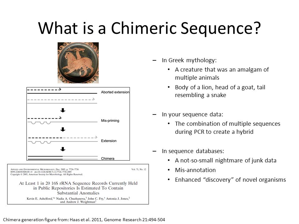
During PCR amplification, it is possible that two unrelated templates are combined to form a sort of hybrid sequence, also called a chimera. Needless to say, we do not want such sequencing artefacts confounding our results. We’ll do this chimera removal using the VSEARCH algorithm that is called within mothur, using the Chimera.vsearch tool.

1. Chimera.vsearch Tool with the following parameters:
   • fasta: the fasta output from Pre.cluster tool
   • Select Reference Template from: Self
   • count: the count table from the last Pre.cluster tool
   • dereplicate: Yes

   Running Chimera.vsearch with the count file will remove the chimeric sequences from the count table, but we still need to remove those sequences from the fasta file as well.

2. Remove.seqs Tool with the following parameters:
   • accnos: the vsearch.accnos file from Chimera.vsearch tool
   • fasta: the fasta output from Pre.cluster tool
   • count: the count table from Chimera.vsearch

Question

1. How many sequences were flagged as chimeric? what is the percentage?

Looking at the chimera.vsearch accnos output, we see that 3,439 representative sequences were flagged as chimeric.

If we run summary.seqs on the resulting fasta file and count table, we see that we went from 128,655 sequences down to 118,091 total sequences in this step, for a reduction of 10,564 total sequences, or 8.2%. This is a reasonable number of sequences to be flagged as chimeric.

Go Up

Taxonomic Classification

Now that we have thoroughly cleaned our data, we are finally ready to assign a taxonomy to our sequences.

We will do this using a Bayesian classifier (via the Classify.seqs tool) and a mothur-formatted training set provided by the Schloss lab based on the RDP (Ribosomal Database Project, Cole et al. 2013) reference taxonomy.

NOTE! In this tutorial we will use the RDP classifier and reference taxonomy for classification, but there are several different taxonomic assignment algorithms and reference databases available for this purpose.

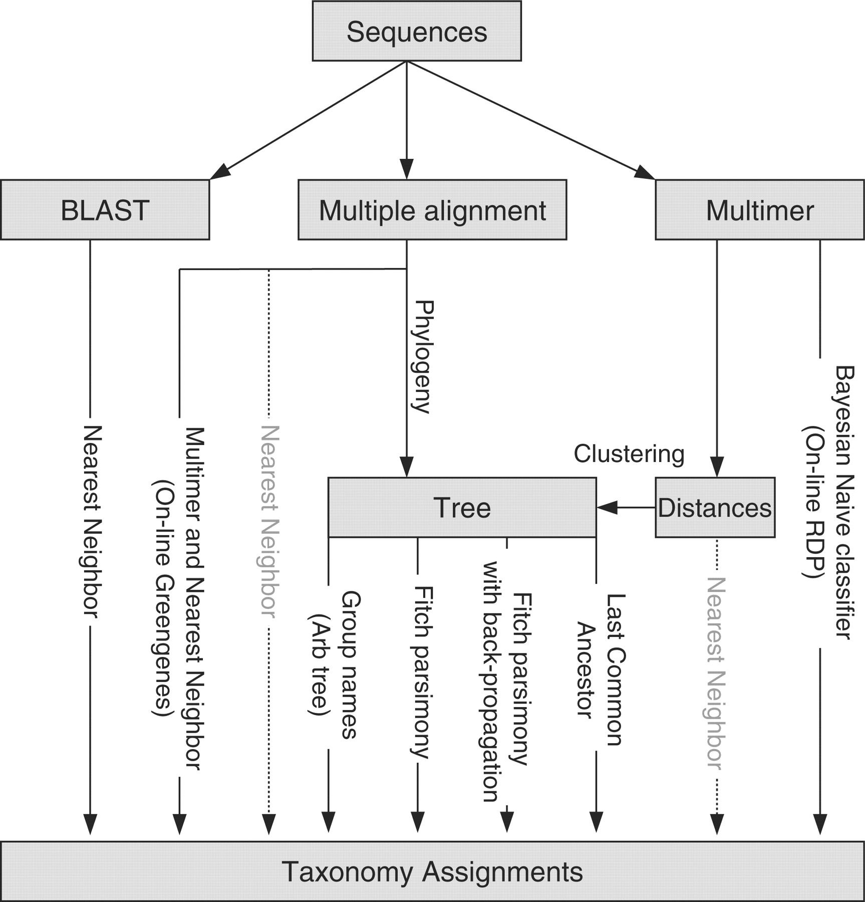
The most commonly used reference taxonomies are:

• SILVA (Quast et al. 2012)
• GreenGenes (DeSantis et al. 2006)
• RDP (Cole et al. 2013)
• NCBI Taxonomy Database (Federhen 2011)

Which reference taxonomy is best for your experiments depends on a number of factors such as the type of sample and variable region sequenced.

Another discussion about how these different databases compare was described by Balvočiūtė and Huson 2017.

Go Up

Removal of non-bacterial sequences

Despite all we have done to improve data quality, there may still be more to do: there may be 18S rRNA gene fragments or 16S rRNA from Archaea, chloroplasts, and mitochondria that have survived all the cleaning steps up to this point.

We are generally not interested in these sequences and want to remove them from our dataset

1. Classify.seqs Tool with the following parameters
   • fasta: the fasta output from Remove.seqs tool
   • reference: trainset9032012.pds.fasta from your history
   • taxonomy: trainset9032012.pds.tax from your history
   • count: the count table file from Remove.seqs
2. Remove.lineage Tool with the following parameters
   • taxonomy: the taxonomy output from Classify.seqs tool
   • taxon - Manually select taxons for filtering: Chloroplast-Mitochondria-unknown-Archaea-Eukaryota
   • fasta: the fasta output from Remove.seqs tool
   • count: the count table from Remove.seqs

Question

1. How many unique (representative) sequences were removed in this step?
2. How many sequences in total?

The data is now as clean as we can get it.

Go Up

Calculate error rates based on our mock community (optional)

This step is only possible if you have co-sequenced a mock community with your samples. A mock community is a sample of which you know the exact composition and is something we recommend to do, because it will give you an idea of how accurate your sequencing and analysis protocol is.

What is a mock community?

A mock community is an artificially constructed sample; a defined mixture of microbial cells and/or viruses or nucleic acid molecules created in vitro to simulate the composition of a microbiome sample or the nucleic acid isolated therefrom.

Why sequence a mock community?

In a mock community, we know exactly which sequences/organisms we expect to find, and at which proportions.

Therefore, we can use such an artificial sample to assess the error rates of our sequencing and analysis pipeline.

• Did we miss any of the sequences we know to be present in the sample (false negatives)?
• Do we find any sequences that were not present in the sample (false positives)?
• Were we able to accurately detect their relative abundances?

If our workflow performed well on the mock sample, we have more confidence in the accuracy of the results on the rest of our samples.

The mock community in this experiment was composed of genomic DNA from 21 bacterial strains. So in a perfect world, this is exactly what we would expect the analysis to produce as a result.

Go Up

Extract mock sample from our dataset

1. Get.groups Tool with the following parameters
   • group file or count table: the count table from Remove.lineage tool
   • groups: Mock
   • fasta: fasta output from Remove.lineage tool
   • output logfile?: yes
2. View the log output

     Selected 58 sequences from your fasta file.
     Selected 4046 sequences from your count file.
   

   The Mock sample has 58 unique sequences, representing a total of 4,046 total sequences.

Go Up

Assess error rates based on a mock community

The Seq.error tool measures the error rates using our mock reference. Here we align the reads from our mock sample back to their known sequences, to see how many fail to match.

1. Seq.error Tool with the following parameters
   • fasta: the fasta output from Get.groups tool
   • reference: HMP_MOCK.v35.fasta file from your history
   • count: the count table from Get.groups tool
   • output log?: yes
2. View the log output

   Overall error rate:    6.5108e-05
   Errors    Sequences
   0    3998
   1    3
   2    0
   3    2
   4    1
   [..]
   

   That is pretty good! The error rate is only 0.0065%! This gives us confidence that the rest of the samples are also of high quality, and we can continue with our analysis.

Go Up

Cluster mock sequences into OTUs

We will now estimate the accuracy of our sequencing and analysis pipeline by clustering the Mock sequences into OTUs, and comparing the results with the expected outcome.

For this a distance matrix is calculated (i.e. the distances between all pairs of sequences). From this distance matrix a clustering is derived using the OptiClust algorithm:

1. OptiClust starts with a random OTU clustering
2. Then iteratively sequences are moved to all other OTUs or new clusters and the option is chosen that improved the mathews correlation coefficient (MCC)
3. Step 2 is repeated until the MCC converges

Let’s Run

1. Dist.seqs Tool the following parameters
   • *fasta: the fasta from Get.groups tool
   • cutoff: 0.20
2. Cluster - Assign sequences to OTUs Tool with the following parameters
   • column: the dist output from Dist.seqs tool
   • count: the count table from Get.groups tool

   Now we make a shared file that summarizes all our data into one handy table

3. Make.shared Tool with the following parameters
   • list: the OTU list from Cluster - Assign sequences to OTUs tool
   • count: the count table from Get.groups tool
   • label: 0.03 (this indicates we are interested in the clustering at a 97% identity threshold)

   And now we generate intra-sample rarefaction curves

4. Rarefaction.single Tool with the following parameters
   • shared: the shared file from Make.shared

Question

1. How many OTUs were identified in our mock community?

Open the rarefaction output (dataset named sobs inside the rarefaction curves output collection), it should look something like this:

numsampled  0.03-	lci-        hci-
1           1.0000	1.0000      1.0000
100         18.1230	16.0000     20.0000
200         19.2930	18.0000     21.0000
300         19.9460	18.0000     22.0000
400         20.4630	19.0000     23.0000
500         20.9330	19.0000     24.0000
600         21.3830	19.0000     24.0000
700         21.8280	19.0000     25.0000
800         22.2560	20.0000     26.0000
900         22.6520	20.0000     26.0000
1000        23.0500	20.0000     27.0000
1100	    23.4790	20.0000     27.0000
1200	    23.8600	21.0000     28.0000
1300	    24.2400	21.0000     28.0000
1400	    24.6210	21.0000     28.0000
1500	    24.9980	22.0000     29.0000
1600	    25.3890	22.0000     29.0000
1700	    25.7870	22.0000     30.0000
1800	    26.1640	23.0000     30.0000
1900	    26.5590	23.0000     30.0000
2000	    26.9490	23.0000     31.0000
2100	    27.3170	24.0000     31.0000
2200	    27.6720	24.0000     31.0000
2300	    28.0110	24.0000     32.0000
2400	    28.3530	25.0000     32.0000
2500	    28.7230	25.0000     32.0000
2600	    29.1040	26.0000     32.0000
2700	    29.4250	26.0000     33.0000
2800	    29.7860	27.0000     33.0000
2900	    30.1420	27.0000     33.0000
3000	    30.4970	27.0000     33.0000
3100	    30.8070	28.0000     33.0000
3200	    31.1450	28.0000     34.0000
3300	    31.4990	28.0000     34.0000
3400	    31.8520	29.0000     34.0000
3500	    32.1970	29.0000     34.0000
3600	    32.5280	30.0000     34.0000
3700	    32.8290	30.0000     34.0000
3800	    33.1710	31.0000     34.0000
3900	    33.5000	32.0000     34.0000
4000	    33.8530	33.0000     34.0000
4046	    34.0000	34.0000     34.0000

When we use the full set of 4060 sequences, we find 34 OTUs from the Mock community; and with 3000 sequences, we find about 31 OTUs.

In an ideal world, we would find exactly 21 OTUs. Despite our best efforts, some chimeras or other contaminations may have slipped through our filtering steps.

Go Up

OTU Clustering

Now that we have assessed our error rates we are ready for some real analysis.

Remove Mock Sample

Now that we have cleaned up our data set as best we can, and assured ourselves of the quality of our sequencing pipeline by considering a mock sample, we are almost ready to cluster and classify our real data.

But before we start, we should first remove the Mock dataset from our data, as we no longer need it.

1. Remove.groups Tool with the following parameters
   • Select input type: fasta , name, taxonomy, or list with a group file or count table
   • *group or count table: the pick.count_table output from Remove.lineage tool
   • groups: Mock
   • fasta: the pick.fasta output from Remove.lineage tool
   • taxonomy: the pick.taxonomy output from Remove.lineage

Go Up

Cluster sequences into OTUs

There are several ways we can perform clustering. For the Mock community, we used the traditional approach of using the Dist.seqs and Cluster tools.

Alternatively, we can also use the Cluster.split tool. With this approach, the sequences are split into bins, and then clustered with each bin. Taxonomic information is used to guide this process.

The Schloss lab have published results showing that if you split at the level of Order or Family, and cluster to a 0.03 cutoff, you’ll get just as good of clustering as you would with the “traditional” approach.

In addition, this approach is less computationally expensive and can be parallelized, which is especially advantageous when you have large datasets.

1. Cluster.split Tool with the following parameters
   • Split by: Classification using fasta
   • fasta: the fasta output from Remove.groups tool
   • taxonomy: the taxonomy output from Remove.groups tool
   • name file or count table: the count table output from Remove.groups tool
   • *taxlevel: 4
   • cutoff: 0.03

   Next we want to know how many sequences are in each OTU from each group and we can do this using the Make.shared tool. Here we tell mothur that we’re really only interested in the 0.03 cutoff level

2. Make.shared Tool with the following parameters
   • list: the list output from Cluster.split tool
   • count: the count table from Remove.groups tool
   • label: 0.03

   We probably also want to know the taxonomy for each of our OTUs.

3. Classify.otu Tool with the following parameters
   • list: the list output from Cluster.split tool
   • count: the count table from Remove.groups tool
   • taxonomy: the taxonomy output from Remove.groups tool
   • label: 0.03

OTU     Size	Taxonomy
...
Otu008  5260	Bacteria(100);"Bacteroidetes"(100);"Bacteroidia"(100);"Bacteroidales"(100);"Rikenellaceae"(100);Alistipes(100);
Otu009	3605	Bacteria(100);"Bacteroidetes"(100);"Bacteroidia"(100);"Bacteroidales"(100);"Porphyromonadaceae"(100);"Porphyromonadaceae"_unclassified(100);
Otu010	3058	Bacteria(100);Firmicutes(100);Bacilli(100);Lactobacillales(100);Lactobacillaceae(100);Lactobacillus(100);
Otu011	2935	Bacteria(100);"Bacteroidetes"(100);"Bacteroidia"(100);"Bacteroidales"(100);"Porphyromonadaceae"(100);"Porphyromonadaceae"_unclassified(100);
Otu012	2078	Bacteria(100);"Bacteroidetes"(100);"Bacteroidia"(100);"Bacteroidales"(100);"Porphyromonadaceae"(100);"Porphyromonadaceae"_unclassified(100);
Otu013	1856	Bacteria(100);Firmicutes(100);Bacilli(100);Lactobacillales(100);Lactobacillaceae(100);Lactobacillus(100);
Otu014	1455	Bacteria(100);Firmicutes(100);Clostridia(100);Clostridiales(100);Lachnospiraceae(100);Lachnospiraceae_unclassified(100);
Otu015	1320	Bacteria(100);Firmicutes(100);Clostridia(100);Clostridiales(100);Lachnospiraceae(100);Lachnospiraceae_unclassified(100);
Otu016	1292	Bacteria(100);Firmicutes(100);Erysipelotrichia(100);Erysipelotrichales(100);Erysipelotrichaceae(100);Turicibacter(100);

The first line shown in the snippet above indicates that Otu008 occurred 5260 times, and that all of the sequences (100%) were binned in the genus Alistipes.

Question

1. Which samples contained sequences belonging to an OTU classified as Staphylococcus? (tax.summary)

Go Up

Subsampling

Before we continue, let’s remind ourselves what we set out to do. Our original question was about the stability of the microbiome and whether we could observe any change in community structure between the early and late samples.

Because some of our sample may contain more sequences than others, it is generally a good idea to normalize the dataset by subsampling.

1. Count.groups Tool with the following parameters
   • shared: the shared file from Make.shared

   Question

   • How many sequences did the smallest sample consist of?
2. Sub.sample Tool with the following parameters
   • Select type of data to subsample: OTU Shared
   • shared: the shared file from Make.shared tool
   • size: 2389

All groups (samples) should now have 2389 sequences. Run count.groups again on the shared output collection by the sub.sample tool to confirm that this is indeed what happened.

Go Up

Diversity Analysis

Species diversity is a valuable tool for describing the ecological complexity of a single sample (alpha diversity) or between samples (beta diversity).

However, diversity is not a physical quantity that can be measured directly, and many different metrics have been proposed to quantify diversity (Finotello et al. 2016).

Species diversity consists of three components: species richness, taxonomic or phylogenetic diversity and species evenness.

• Species richness = the number of different species in a community.
• Species evenness = how even in numbers each species in a community is.
• Phylogenetic diversity = how closely related the species in a community are.

Go Up

Alpha diversity

In order to estimate alpha diversity of the samples, we first generate the rarefaction curves.

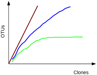
Recall that rarefaction measures the number of observed OTUs as a function of the subsampling size.

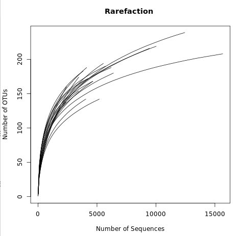
A rarefaction curve plots the number of species as a function of the number of individuals sampled. The curve usually begins with a steep slope, which at some point begins to flatten as fewer species are being discovered per sample: the gentler the slope, the less contribution of the sampling to the total number of operational taxonomic units or OTUs.

• Green -> most or all species have been sampled;
• Blue -> this habitat has not been exhaustively sampled;
• Red -> species rich habitat, only a small fraction has been sampled.

Go Up

Calculate Rarefaction

1. Rarefaction.single Tool with the following parameters
   • shared: the shared file from Make.shared

Note that we used the default diversity measure here (sobs; observed species richness), but there are many more options available under the calc parameter. Descriptions of some of these calculators can be found on the mothur wiki.

Examine the rarefaction curve output.

numsampled    0.03-F3D0    lci-F3D0    hci-F3D0    0.03-F3D1   ...
1              1.0000       1.0000      1.0000      1.0000
100           41.6560      35.0000     48.0000     45.0560
200           59.0330      51.0000     67.0000     61.5740
300           70.5640      62.0000     79.0000     71.4700
400           78.8320      71.0000     87.0000     78.4730
500           85.3650      77.0000     94.0000     83.9990
...

This file displays the number of OTUs identified per amount of sequences used (numsampled). What we would like to see is the number of additional OTUs identified when adding more sequences reaching a plateau.

Then we know we have covered our full diversity. This information would be easier to interpret in the form of a graph.

Go Up

Plot Rarefaction

1. Plotting tool - for multiple series and graph types Tool with the following parameters
   • Plot Title: Rarefaction
   • Label for x axis: Number of Sequences
   • Label for y axis: Number of OTUs
   • Output File Type: PNG
   • Click on Insert Series:
     • Dataset: rarefaction curve collection
     • Header in first line?: Yes
     • Column for x axis: Column 1
     • Column for y-axis: Column 2 and Column 5 and every third column until the end (we are skipping the low confidence and high confidence interval columns)

   View the rarefaction plot output. From this image can see that the rarefaction curves for all samples have started to level off so we are confident we cover a large part of our sample diversity:

   

Go Up

Summary.single

Finally, let’s use the Summary.single tool to generate a summary report. The following step will randomly subsample down to 2389 sequences, repeat this process 1000 times, and report several metrics:

1. Summary.single Tool with the following parameters
   • share: the shared file from Make.shared tool
   • calc: nseqs,coverage,sobs,invsimpson
   • size: 2389

View the summary output from Summary.single tool. This shows several alpha diversity metrics:

• sobs: observed richness (number of OTUs)
• coverage: Good’s coverage index (1 - (number of OTUs containing a single sequence / total number of sequences ))
• invsimpson: Inverse Simpson Index (1 / probability that two random individuals represent the OTU)
• nseqs: number of sequences

label   group   sobs          coverage    invsimpson   invsimpson_lci   invsimpson_hci  nseqs
0.03    F3D0    167.000000    0.994697    25.686387    24.648040        26.816067       6223.000000
0.03    F3D1    145.000000    0.994030    34.598470    33.062155        36.284520       4690.000000
0.03    F3D141  154.000000    0.991060    19.571632    18.839994        20.362390       4698.000000
0.03    F3D142  141.000000    0.978367    17.029921    16.196090        17.954269       2450.000000
0.03    F3D143  135.000000    0.980738    18.643635    17.593785        19.826728       2440.000000
0.03    F3D144  161.000000    0.980841    15.296728    14.669208        15.980336       3497.000000
0.03    F3D145  169.000000    0.991222    14.927279    14.494740        15.386427       5582.000000
0.03    F3D146  161.000000    0.989167    22.266620    21.201364        23.444586       3877.000000
0.03    F3D147  210.000000    0.995645    15.894802    15.535594        16.271013       12628.000000
0.03    F3D148  176.000000    0.995725    17.788205    17.303206        18.301177       9590.000000
0.03    F3D149  194.000000    0.994957    21.841083    21.280343        22.432174       10114.000000
0.03    F3D150  164.000000    0.989446    23.553161    22.462533        24.755101       4169.000000
0.03    F3D2    179.000000    0.998162    15.186238    14.703161        15.702137       15774.000000
0.03    F3D3    127.000000    0.994167    14.730640    14.180453        15.325243       5315.000000
0.03    F3D5    138.000000    0.990523    29.415378    28.004777        30.975621       3482.000000
0.03    F3D6    155.000000    0.995339    17.732145    17.056822        18.463148       6437.000000
0.03    F3D7    126.000000    0.991916    13.343631    12.831289        13.898588       4082.000000
0.03    F3D8    158.000000    0.992536    23.063894    21.843396        24.428855       4287.000000
0.03    F3D9    162.000000    0.994803    24.120541    23.105499        25.228865       5773.000000

There are a couple of things to note here:

• The differences in diversity and richness between early and late time points is small.
• All sample coverage is above 97%.

There are many more diversity metrics, and for more information about the different calculators available in mothur, see the mothur wiki page

Go Up

Beta diversity

Beta diversity is a measure of the similarity of the membership and structure found between different samples. The default calculator in the following section is thetaYC, which is the Yue & Clayton theta similarity coefficient. We will also calculate the Jaccard index (termed jclass in mothur).

1. Dist.shared Tool with the following parameters
   • shared: to the shared file from Make.shared tool
   • calc: thetayc,jclass
   • subsample: 2389
2. Heatmap.sim Tool with the following parameters
   • Generate Heatmap for: phylip
   • phylip: the output of Dist.shared tool (this is a collection input)

Look at some of the resulting heatmaps (you may have to download the SVG images first). In all of these heatmaps the red colors indicate communities that are more similar than those with black colors.

For example this is the heatmap for the thetayc calculator (output thetayc.0.03.lt.ave):

and the jclass calulator (output jclass.0.03.lt.ave):

Go Up

Venn diagram

When generating Venn diagrams we are limited by the number of samples that we can analyze simultaneously.

Let’s take a look at the Venn diagrams for the first 4 time points of female 3 using the Venn tool:

1. Venn Tool with the following parameters
   • OTU Shared: output from Sub.sample tool (collection)
   • groups: F3D0,F3D1,F3D2,F3D3

This shows that there were a total of 218 OTUs observed between the 4 time points. Only 73 of those OTUs were shared by all four time points. We could look deeper at the shared file to see whether those OTUs were numerically rare or just had a low incidence.

Go Up

Tree

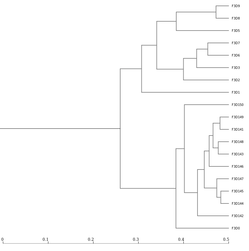
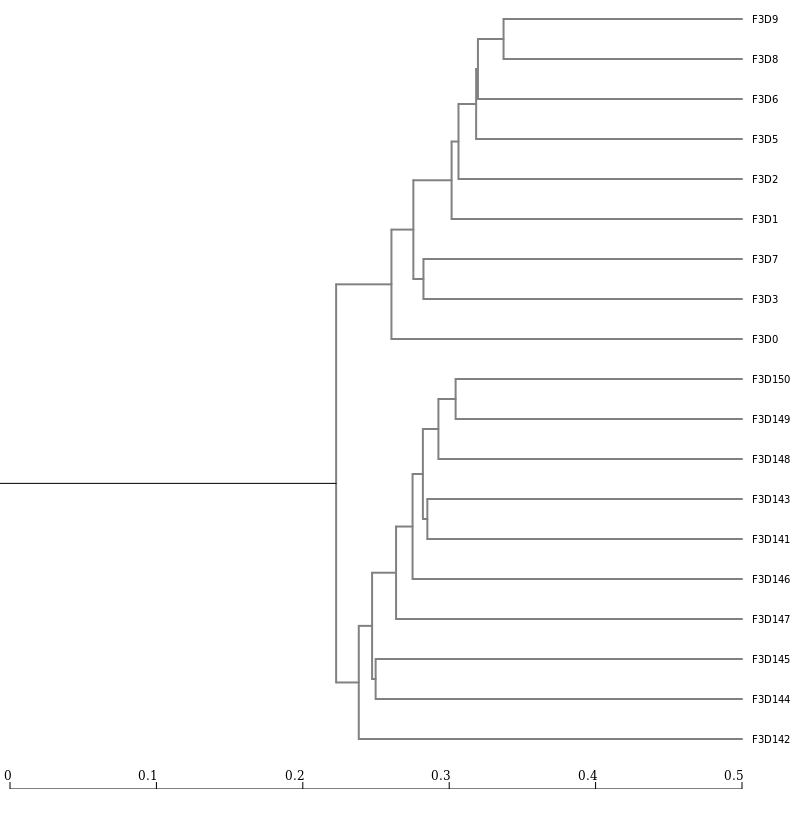
Next, let’s generate a dendrogram to describe the similarity of the samples to each other. We will generate a dendrogram using the jclass and thetayc calculators within the Tree.shared tool:

1. Tree.shared Tool with the following parameters
   • Select input format: Phylip Distance Matrix
   • phylip: the distance files output from Dist.shared
2. Newick display Tool with the following parameters
   • Newick file: output from Tree.shared

Inspection of the tree shows that the early and late communities cluster with themselves to the exclusion of the others.

• thetayc.0.03.lt.ave:
• jclass.0.03.lt.ave:

Go Up

Visualisations

Krona

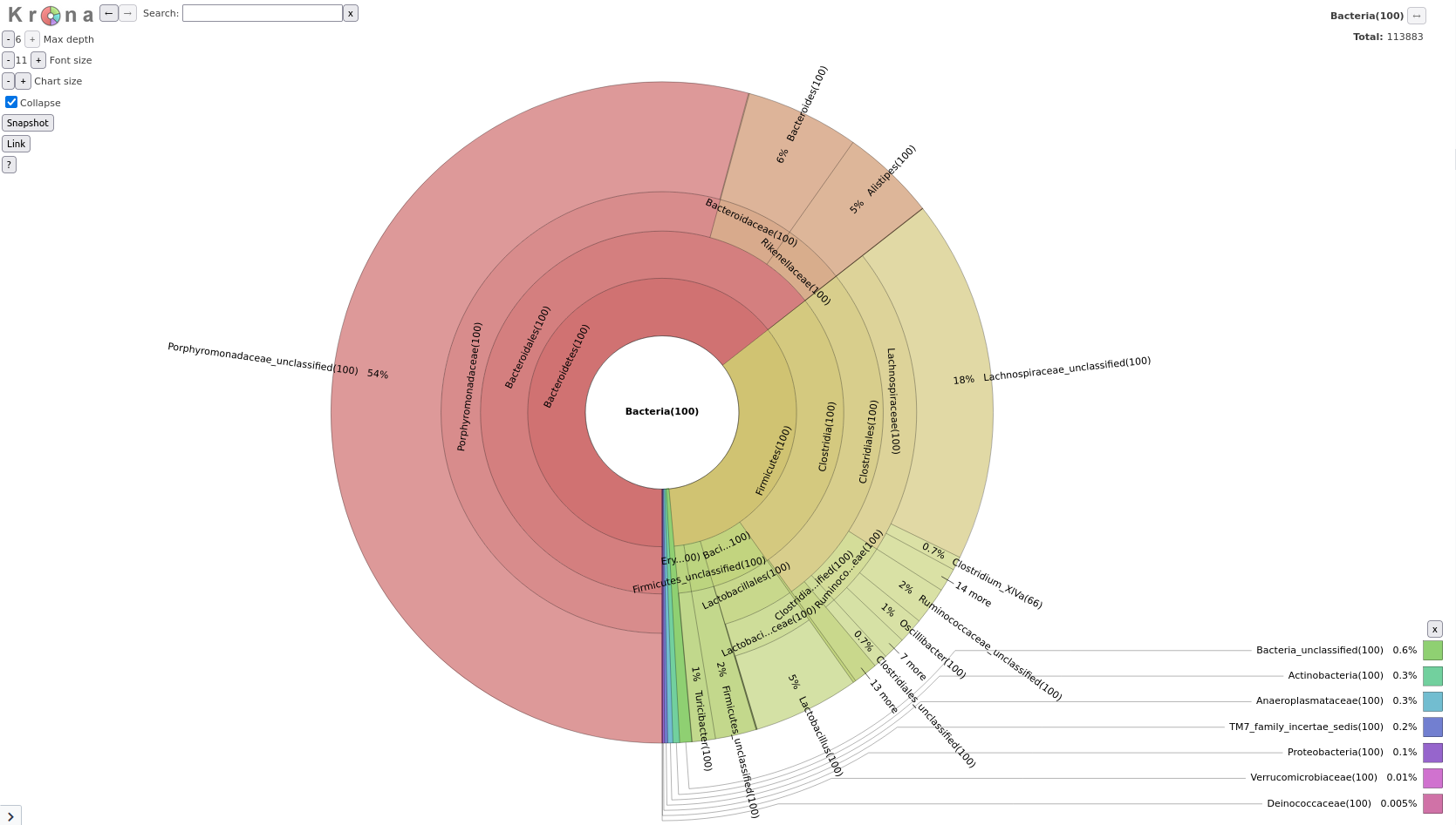
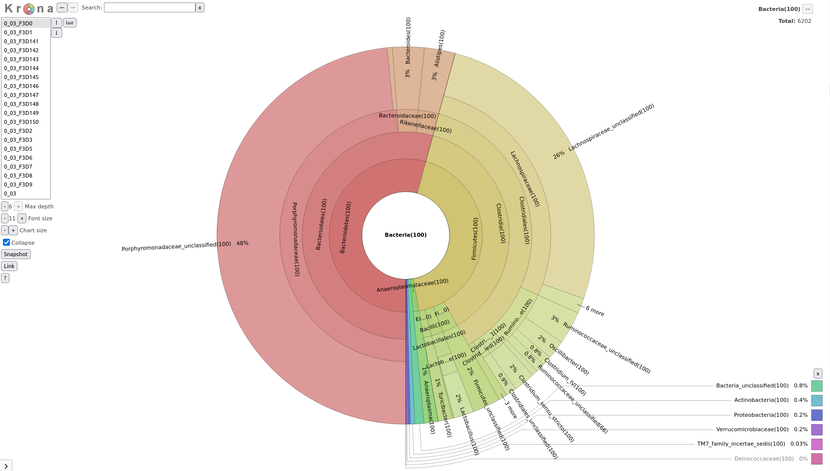
As we saw in the previous lectures, a tool we can use to visualize the composition of our community, is Krona

1. Taxonomy-to-Krona Tool with the following parameters
   • Taxonomy file: the taxonomy output from Classify.otu
2. Krona pie chart Tool with the following parameters
   • Type of input: Tabular
   • Input file: the taxonomy output from Taxonomy-to-Krona

The resulting file is an HTML file containing an interactive visualization. For instance try double-clicking the innermost ring labeled “Bacteroidetes”.

Question

1. What percentage of your sample was labelled Lactobacillus?

Go Up

Generating per-sample Krona plots (Exercise)

1. Re-run the Classify.otu tool we ran earlier
   • list: the list output from Cluster.split tool
   • count: the count table from Remove.groups tool
   • taxonomy: the taxonomy output from Remove.groups tool
   • label: 0.03
   • persample - allows you to find a consensus taxonomy for each group: Yes
2. Taxonomy-to-Krona Tool with the following parameters
   • Taxonomy file: the taxonomy collection from Classify.otu
3. Krona pie chart Tool with the following parameters
   • Type of input: Tabular
   • Input file: the collection from Taxonomy-to-Krona tool
   • Combine data from multiple datasets?: No

The final result should look something like this (switch between samples via the list on the left):

Go Up

Phinch

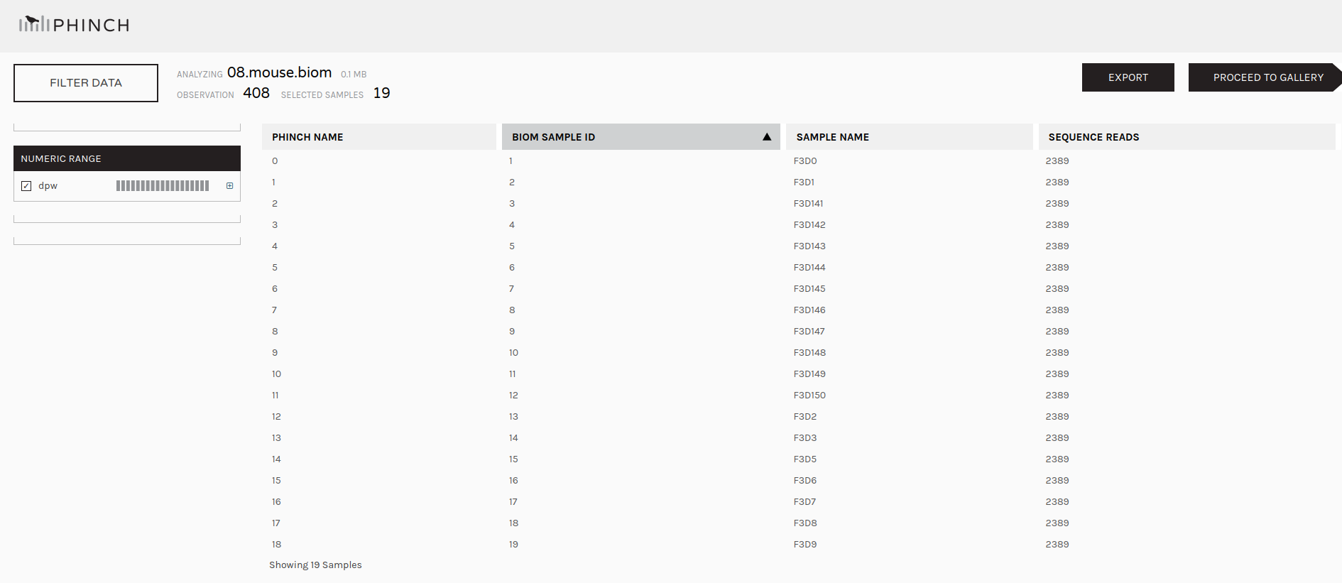
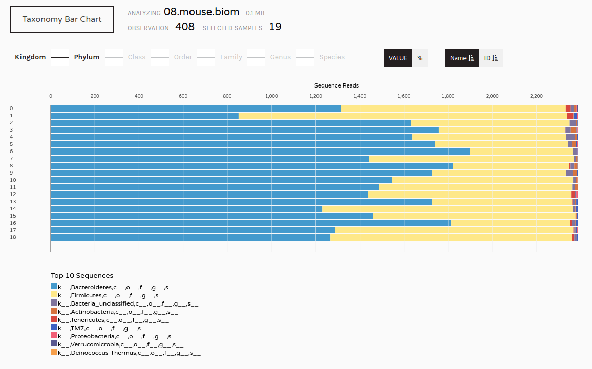
We may now wish to further visualize our results. We can convert our shared file to the more widely used biom format and view it in a platform like Phinch.

1. Make.biom Tool with the following parameters
   • shared: the output from Sub.sample tool (collection)
   • constaxonomy: the taxonomy output from Classify.otu tool
   • metadata: the mouse.dpw.metadata file you uploaded at the start of this tutorial
2. Download the generated BIOM file from Galaxy
3. Upload it directly to the Phinch server at https://usegalaxy.eu/phinch/.

Important: After downloading, please change the file extension from .biom1 to .biom before uploading to Phinch.

Go Up

Conclusion

• 16S rRNA gene sequencing analysis results depend on the many algorithms used and their settings
• Quality control and cleaning of your data is a crucial step in order to obtain optimal results
• Adding a mock community to serve as a control sample can help you asses the error rate of your experimental setup
• We can explore alpha and beta diversities using Krona and Phinch for dynamic visualizations

Go Up