Genomic Data Visualisation with JBrowse

How can I visualise features or blast data? How can I visualise sequencing data in a workflow? Build several visualisations in JBrowse. Have basic familiarity with moving around JBrowse, and loading several data tracks


JBrowse is a fast, embeddable genome browser built completely with JavaScript and HTML5, with optional run-once data formatting tools written in Perl.

The Galaxy tool accepts data in many formats:

  • Intervals/Annotation/Feature Tracks (GFF/GFF3, BED, GenBank)
  • BAM Pileups
  • Blast XML results
  • Wig/BigWig
  • VCF files

The JBrowse tool has an incredibly extensive number of options, more than anyone needs most of the time.


Data Upload

The data for today is a subset of real datasets from E. coli MG1655 strain K-12

  1. Create and name a new history.

  2. Import the datasets:

    https://zenodo.org/record/3591856/files/blastp%20genes.gff3
    https://zenodo.org/record/3591856/files/blastp%20vs%20swissprot.xml
    https://zenodo.org/record/3591856/files/dna%20sequencing.bam
    https://zenodo.org/record/3591856/files/dna%20sequencing%20coverage.bw
    https://zenodo.org/record/3591856/files/genes%20(de%20novo).gff3
    https://zenodo.org/record/3591856/files/genes%20(NCBI).gff3
    https://zenodo.org/record/3591856/files/genome.fa
    https://zenodo.org/record/3591856/files/RNA-Seq%20coverage%201.bw
    https://zenodo.org/record/3591856/files/RNA-Seq%20coverage%202.bw
    https://zenodo.org/record/3591856/files/variants.vcf
    

Go Up


Simple Gene Tracks

  • We will start by adding a couple of gene call tracks.
  • In our case these are genes and gene predictions, but they don’t have to be.
  • In the general case this can be any interesting region from an analysis, where a tool has pointed out some region for further inspection for some reason, then this data can be visualised with the “gene” track type.
  1. JBrowse Tool with the following parameters:
    • Reference genome to display: Use a genome from history
      • Select the reference genome: genome.fa
    • Genetic Code: 11. The Bacterial, Archaeal and Plant Plastid Code
    • In Track Group:
      • Insert Track Group
        • Track Category: Genes
        • In Annotation Track:
          • Track Type: GFF/GFF3/BED Features
            • GFF/GFF3/BED Track Data: genes (de novo).gff3
  2. Execute
  3. View the contents of the file

  • Tracks are shown on the left. Clicking the checkboxes will make the tracks visible or invisible
  • You can use your mouse scrollwheel to move around the genome view area, or you can click and drag to move.
  • Double clicking will zoom in on the genome, or you can use the magnifying glass icons to zoom in our out

  • The JBrowse tool takes track names directly from file names
  • If you want to rename tracks: Click on the pencil icon, edit the Name and click Save
  • You can now re-run the JBrowse tool and it will produce a new JBrowse instance with corrected names.

Go Up


Complex Gene Tracks

All of the track types in the JBrowse tool support a wide array of features. We’ve only looked at a simple track with default options, however there are more tools available to us to help create user-friendly JBrowse instances that can embed rich data.

  1. JBrowse with the following parameters:
    • Reference genome to display: Use a genome from history
      • Select the reference genome: genome.fa
    • Genetic Code: 11. The Bacterial, Archaeal and Plant Plastid Code
    • In Track Group:
      • Insert Track Group
        • Track Category: Genes
        • In Annotation Track:
          • Insert Annotation Track
            • Track Type: GFF/GFF3/BED Features
              • GFF/GFF3/BED Track Data: genes (de novo).gff3
              • JBrowse Track Type [Advanced]: Canvas Features
              • In JBrowse Feature Score Scaling & Coloring Options [Advanced]:
                • Color Score Algorithm: Based on score
                  • How should minimum and maximum values be determined for the scores of the features: Manually specify minimum and maximum expected scores for the feature track
                    • Minimum expected score: 0
                    • Maximum expected score: 1
          • Insert Annotation Track
            • Track Type: GFF/GFF3/BED Features
              • GFF/GFF3/BED Track Data: genes (NCBI).gff3
              • JBrowse Track Type [Advanced]: Canvas Features
                • In JBrowse Contextual Menu options [Advanced]:
                  • In Track Menu:
                    • Insert Track Menu
                      • Menu label: See protein at NCBI
                      • Menu url: https://www.ncbi.nlm.nih.gov/gene?term={locus_tag}%5BGene%20Name%5D
                      • Menu icon: Database
  2. View the output. The lighter coloured genes on the denovo track are coloured based on the confidence score given to the prediction by AUGUSTUS. NCBI genes do not have scores, these are more like an official gene set.

  3. Turn on both tracks of data
  4. Navigate to 21,200, either manually, or by copying and pasting the location block: NC_000913.3:18351..24780
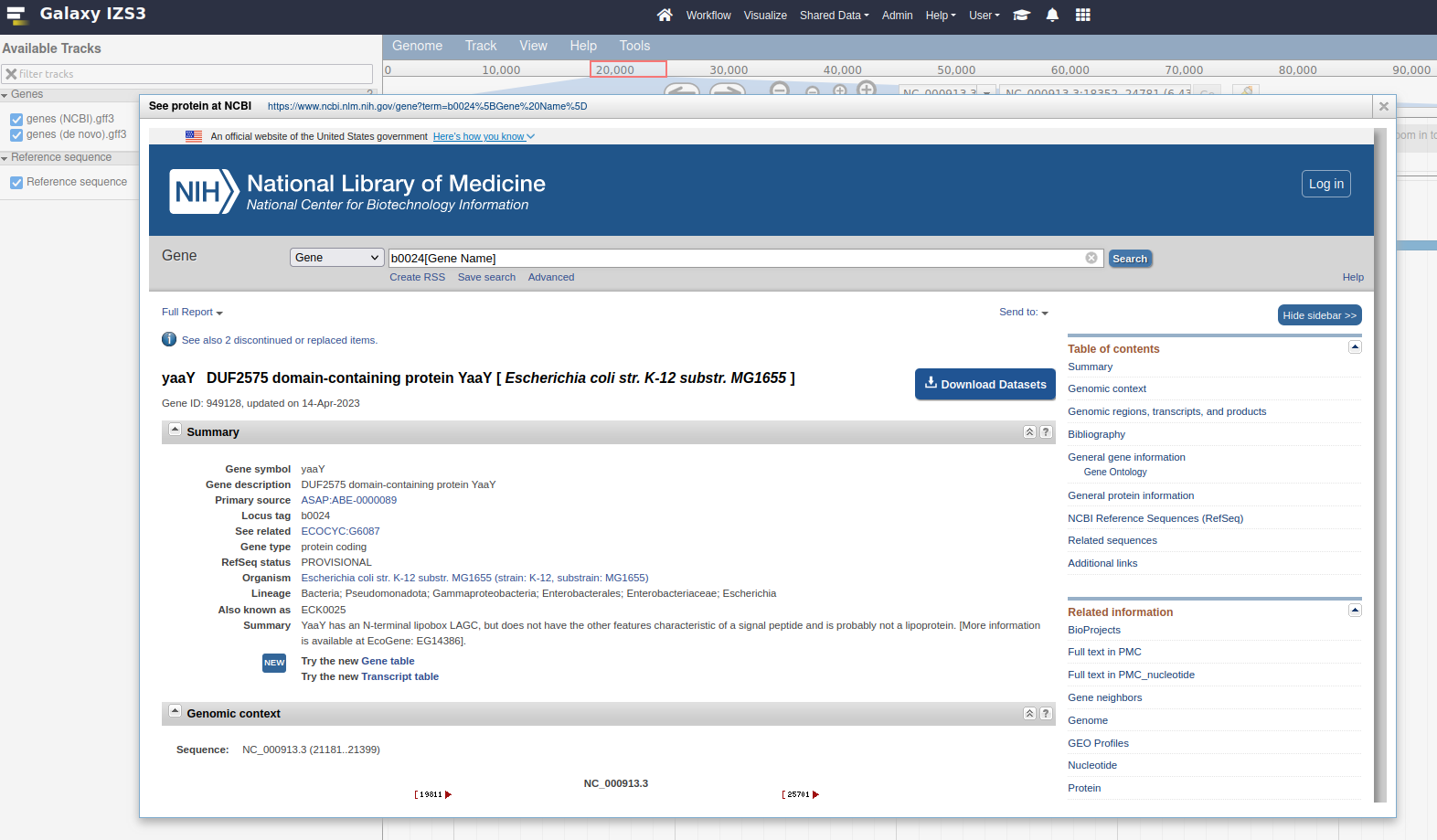
  5. Right click on the yaaY gene, and click the See protein at NCBI menu option. This menu option is dynamic, try it with a few other features from the genes (NCBI).gff3 track. These features have a locus_tag and the menu button we added will open a URL to an NCBI search page for the value of this locus_tag attribute

Contextual Menu

In JBrowse terminology the right click menu of some features is called the contextual menus.

You can customize this menu to add new links and options that will be useful to the user. These links can be templated with variables based on metadata of the feature that the user clicked upon.

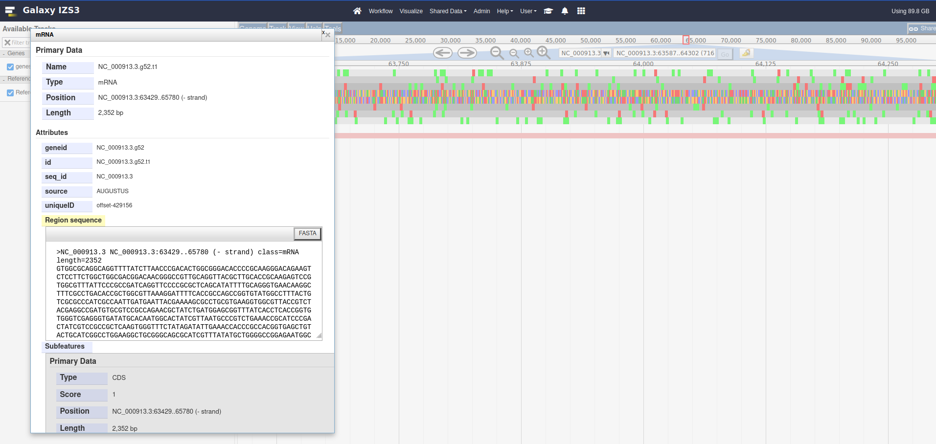
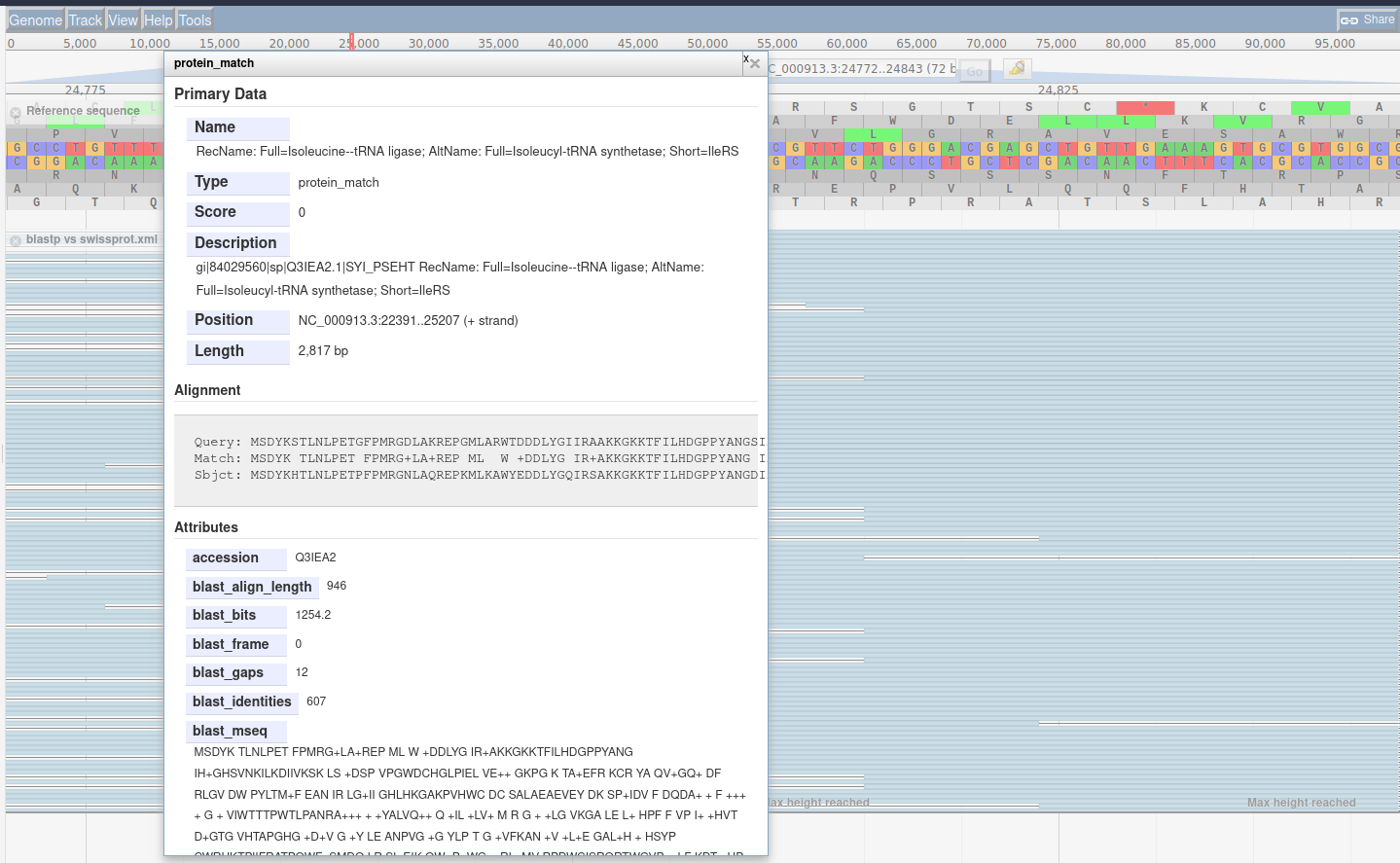
There are more valid values for templating than mentioned in the help. When you click on a feature in the JBrowse instance, it will present all of the properties of the feature. Any of the top level properties can be used directly in your templating

Contextual menus can be used to link to more than just NCBI.

  • The links can go anywhere such as web search services (e.g. Google) or genomics web services (e.g. EBI)
  • Some sites use the IFrame action to link genes to local services where users are expected to submit annotation notes or data.

Go Up


Sequencing, Coverage, and Variation

This is the next major category of data that people wish to visualize: sequencing, coverage, and variation.

  1. The sequencing data can be of any type, and does not necessarily need to be sequencing data, as long as the results are formatted as BAM files.

  2. Here we will add several coverage tracks (essentially a line plot along the genome, associating a position with a value) with various visualisation options like scaling and display type. Each of these visualisation options can be useful in different situations, but it largely is a matter of preference or what you are used to seeing.

  3. Next we will add a sequencing dataset, a BAM file which maps some sequencing reads against various locations along the genome. JBrowse helpfully highlights which reads have mapping issues, and any changes in bases between the reads and the genome.

  4. We Autogenerate a SNP track, which produces an extra track we can enable in JBrowse. This track reads the same BAM file used for visualising reads, and then produces a SNP and coverage visualisation.

NB: This only works for small BAM files, if your files are large (>200 Mb), then you should consider generating these coverage and SNP tracks by other means (e.g. bamCoverage and FreeBayes or similar tools) as it will be significantly faster.

  1. JBrowse with the following parameters:
    • Reference genome to display: Use a genome from history
      • Select the reference genome: genome.fa
      • Genetic Code: 11. The Bacterial, Archaeal and Plant Plastid Code
      • In Track Group:
        • Insert Track Group
          • Track Category: Coverage
          • In Annotation Track:
            • Insert Annotation Track
              • Track Type: BigWig XY
              • BigWig Track Data: dna sequencing coverage.bw
            • Insert Annotation Track
              • Track Type: BigWig XY
              • BigWig Track Data: rna-seq coverage/1.bw
              • Use XYPlot: Yes
            • Insert Annotation Track
              • Track Type: BigWig XY
              • BigWig Track Data: rna-seq coverage/2.bw
              • Use XYPlot: Yes
              • Show variance band: Yes
              • Track Scaling: Autoscale (global)
        • Insert Track Group
          • Track Category: Sequencing & Variation
          • In Annotation Track:
            • Insert Annotation Track
              • Track Type: BAM Pileups
                • BAM Track Data: sequencing.bam
                • Autogenerate SNP Track: Yes
            • Insert Annotation Track
              • Track Type: VCF SNPs
                • SNP Track Data: variants.vcf
  2. Execute and then explore the resulting data.
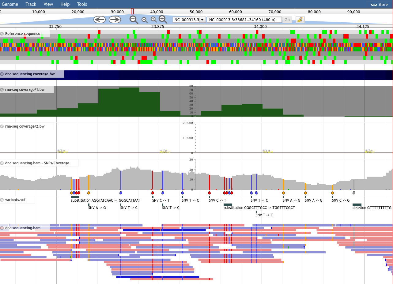
  3. Try:

    • Clicking on individual variations in the dedicated variants.vcf track
    • Hovering over the autogenerated SNPs/Coverage track
    • Clicking on individual reads of the sequencing.bam track
    • Changing the visualisation options of the BAM track

Go Up


Blast Results

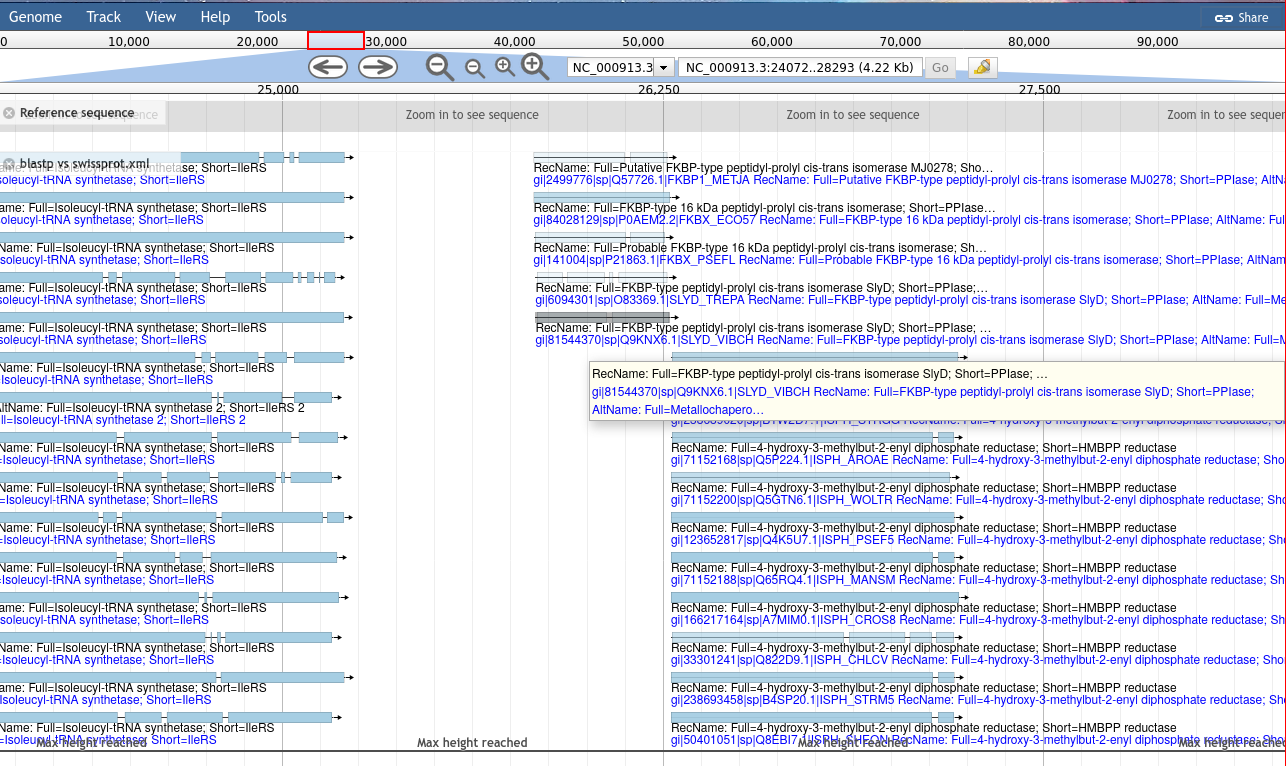
The Blast visualisation module requires that you have a gff3 formatted set of features which you then exported as DNA or protein, and blasted.

The reason is easy to understand: when you extract DNA/protein sequences for Blasting, this process looses information about where these sequences were along the genome. The results from Blast retains the identifiers from the DNA/protein sequences, so we need to map these identifiers, to proper features with locations.

The best way to accomplish this is through the gffread tool which can cleanup a gff3 file, and export various features, optionally translating them.

With these outputs, the cleaned features and fasta formatted sequences, you can Blast the sequences, and then supply the resulting Blast XML outputs in addition to the cleaned features, allowing a script to re-associate these Blast results to their original locations along the genome.

  1. JBrowse with the following parameters:
    • Reference genome to display: Use a genome from history
      • Select the reference genome: genome.fa
      • Genetic Code: 11. The Bacterial, Archaeal and Plant Plastid Code
      • In Track Group:
        • Insert Track Group
          • Track Category: BLAST
          • In Annotation Track:
            • Insert Annotation Track
              • Track Type: Blast XML
                • BlastXML Track Data: blastp vs swissprot.xml
                • Features used in Blast Search: blastp genes.gff3
                • Minimum Gap Size: 5
                • Is this a protein blast search?: Yes
                • In JBrowse Feature Score Scaling & Coloring Options [Advanced]:
                  • Color Score Algorithm: Based on score
                    • JBrowse style.color function’s score scaling: Blast scaling
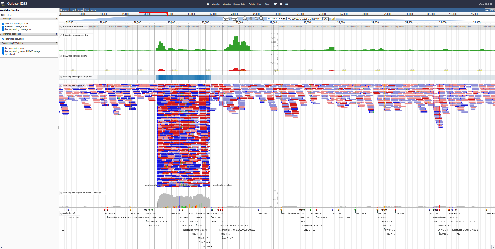
  2. Execute and then explore the resulting data.
Go Up


Conclusion

This does not exhaustively cover JBrowse, and the tool is more extensible than can be easily documented, but hopefully these examples are illustrative and can give you some ideas about it

Go Up