Assembly of metagenomic sequencing data

Why metagenomic data should be assembled? What is the difference between co-assembly and individual assembly? What is the difference between reads, contigs and scaffolds? How to assess the quality of metagenomic data assembly?


Metagenomics involves the extraction, sequencing and analysis of combined genomic DNA from entire microbiome samples. It includes then DNA from many different organisms, with different taxonomic background.

Reconstructing the genomes of microorganisms in the sampled communities is critical step in analyzing metagenomic data. To do that, we can use assembly and assemblers, i.e. computational programs that stich together the small fragments of sequenced DNA produced by sequencing instruments.

For a thorough analysis of the community, metagenomic shotgun reads can be assembled with the help of available reference genomes (reference-based assembly) or de novo (de-novo assembly).

Assembling seems intuitively similar to putting together a jigsaw puzzle.

Ideally, the result of a metagenome assembly process should be a set of genomes of all the species that are represented within the input data. In reality, this end result is still very difficult to achieve.

Metagenomic assembly is further complicated by:

  • the large volume of data produced
  • the quality of the sequence
  • the unequal representation of members of the microbial community
  • the presence of closely related microorganisms with similar genomes
  • the presence of several strains of the same microorganism
  • an insufficient amount of data for minor community members

For assembly, there are 3 main strategies:
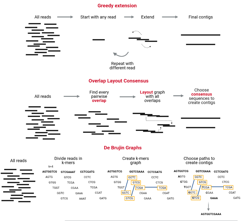
  1. Greedy extension
  2. Overlap Layout Consensus
  3. De Bruijn graphs.

In this tutorial, we will learn how to run metagenomic assembly tool and evaluate the quality of the generated assemblies.

We will use data from the study: Temporal shotgun metagenomic dissection of the coffee fermentation ecosystem.

For an in-depth analysis of the structure and functions of the coffee microbiome, a temporal shotgun metagenomic study (six time points) was performed. The six samples have been sequenced with Illumina MiSeq utilizing whole genome sequencing.

Go Up


Assembly

As explained before, there are many challenges to metagenomics assembly, including:

  1. differences in coverage between samples, resulting from differences in abundance,
  2. the fact that different species often share conserved regions
  3. the presence of multiple strains of a single species

To reduce the differences in coverage between samples, we can use a co-assembly approach, where reads from all samples are aligned together:
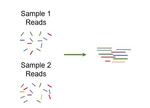
Pros of co-assembly Cons of co-assembly
More data Higher computational overhead
Better/longer assemblies Risk of shattering your assembly
Access to lower abundant organisms Risk of increased contamination

Co-assembly is then not always beneficial:

  • Changes in strain can cause the assembly graph to collapse
  • Binned contigs are likely to be misclassified: MAGs must be treated as a population genom

Co-assembly is reasonable if:

  • Same samples
  • Same sampling event
  • Longitudinal sampling of the same site
  • Related samples

If it is not the case, individual assembly should be preferred. In this case, an extra step of de-replication should be used
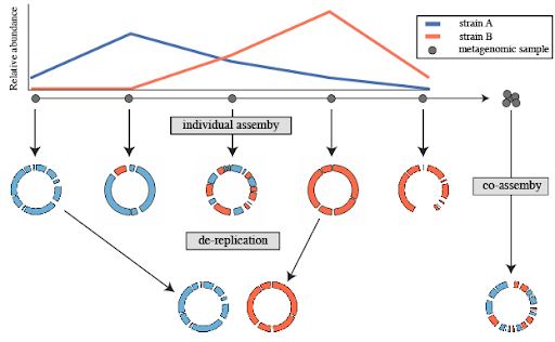
Co-assembly is more commonly used than individual assembly and then de-replication after binning. But in this tutorial, to show all steps, we will run an individual assembly.

NOTE! Sometimes it is important to run assembly tools both on individual samples and on all pooled samples, and use both outputs to get the better outputs for the certain dataset.

Several tools are available for metagenomic assembly. But 2 are the most used ones:

  • MetaSPAdes: a short-read assembler designed specifically for large and complex metagenomics datasets.
    • It is particularly optimal for high-coverage metagenomes
    • with the best contig metrics
    • produces few under-collapsed/over-collapsed repeats
  • MEGAHIT: a single node assembler for large and complex metagenomics NGS reads, such as soil.
    • It is currently the most efficent computationally assembler: it has the lowest memory and time consumption.
    • It produced some of the best assemblies (irrespective of sequencing coverage) with the fewest structural errors
    • outperforms in recovering the genomes of closely related strains
    • but has a bias towards relatively low coverage genomes leading to a suboptimal assembly of high abundant community member genomes in very large datasets

Both tools are available in Galaxy. But currently, only MEGAHIT can be used in individual mode for several samples.

NOTE!! See also Spades and Unicycler

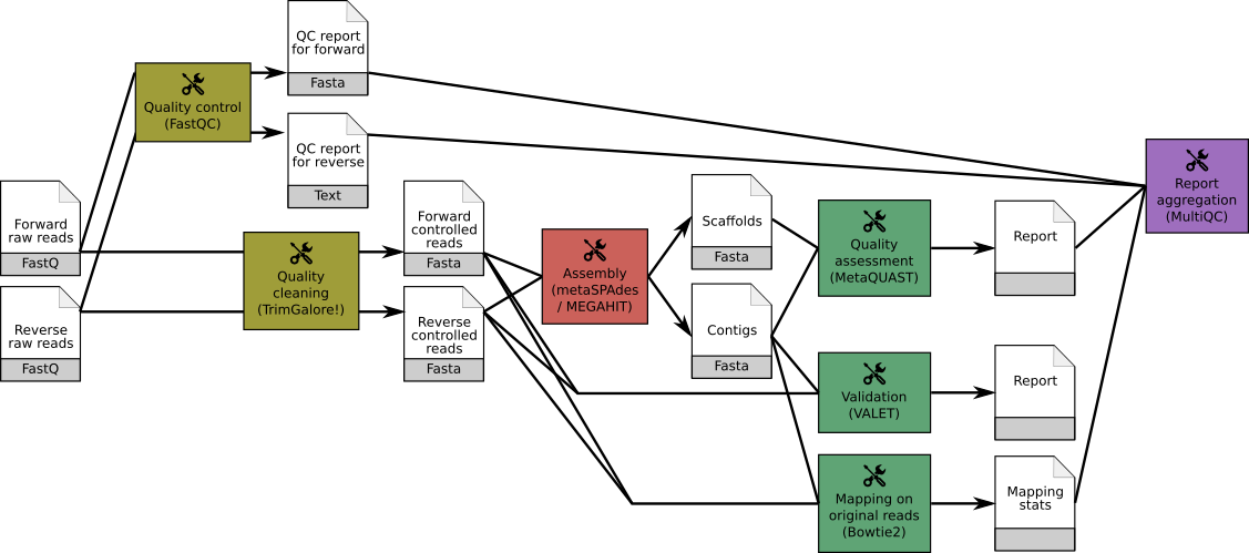
A typical assembly workflow consists of:

  1. Processing with quality control/trimming (FastQC and Trim Galore! or Cutadapt)
  2. Assembly with either MEGAHIT or MetaSPAdes
  3. Estimation of the assembly quality statistics with MetaQUAST or Quast
  4. Identification of potential assembly error signature with VALET
  5. Determination of percentage of unmapped reads with Bowtie2 combined with MultiQC to aggregate the results.
Go Up


Preparing data

NOTE! Please, use:

  1. Create a new history and rename it
  2. Import data
    https://zenodo.org/record/7818827/files/ERR2231567_1.fastqsanger.gz
    https://zenodo.org/record/7818827/files/ERR2231567_2.fastqsanger.gz
    https://zenodo.org/record/7818827/files/ERR2231568_1.fastqsanger.gz
    https://zenodo.org/record/7818827/files/ERR2231568_2.fastqsanger.gz
    https://zenodo.org/record/7818827/files/ERR2231569_1.fastqsanger.gz
    https://zenodo.org/record/7818827/files/ERR2231569_2.fastqsanger.gz
    https://zenodo.org/record/7818827/files/ERR2231570_1.fastqsanger.gz
    https://zenodo.org/record/7818827/files/ERR2231570_2.fastqsanger.gz
    https://zenodo.org/record/7818827/files/ERR2231571_1.fastqsanger.gz
    https://zenodo.org/record/7818827/files/ERR2231571_2.fastqsanger.gz
    https://zenodo.org/record/7818827/files/ERR2231572_1.fastqsanger.gz
    https://zenodo.org/record/7818827/files/ERR2231572_2.fastqsanger.gz 
    
  3. Create a paired collection named Raw reads, rename your pairs with the sample name
    • Click on Select Items at the top of the history panel
    • Check all the datasets in your history you would like to include
    • Click n of N selected and choose Build List of Dataset Pairs
    • Change the text of unpaired forward to a common selector for the forward reads
    • Change the text of unpaired reverse to a common selector for the reverse reads
    • Click Pair these datasets for each valid forward and reverse pair.
    • Enter a name for your collection: Raw Reads
    • Click Create List to build your collection
    • Click on the checkmark icon at the top of your history again

Go Up


Individual assembly with MEGAHIT

  1. MEGAHIT Tool with parameters
    • Select your input option: Paired-end collection
    • Run in batch mode?: Run individually
    • Select a paired collection: Raw reads
    • Basic assembly options
      • K-mer specification method: Specify min, max, and step values
      • Minimum kmer size: 21
      • Maximum kmer size: 91
      • Increment of kmer size of each iteration: 12
  2. Don’t RUN
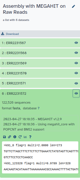
  3. Since the assembly process would take ~1h we are just going to import the results of the assembly previously run.
    https://zenodo.org/record/7818827/files/contigs_ERR2231567.fasta
    https://zenodo.org/record/7818827/files/contigs_ERR2231568.fasta
    https://zenodo.org/record/7818827/files/contigs_ERR2231569.fasta
    https://zenodo.org/record/7818827/files/contigs_ERR2231570.fasta
    https://zenodo.org/record/7818827/files/contigs_ERR2231571.fasta
    https://zenodo.org/record/7818827/files/contigs_ERR2231572.fasta
    
  4. Create a collection named MEGAHIT Contig, rename your pairs with the sample name

MEGAHIT produced a collection of output assemblies - one per sample - that can be proceeded further in binning step and then de-replication.

The output contains contigs, contiguous lengths of genomic sequences in which bases are known to a high degree of certainty.

Contrary to MetaSPAdes, MEGAHIT does not output scaffolds, i.e. segments of genome sequence reconstructed from contigs and gaps.

The gaps occur when reads from the two sequenced ends of at least one fragment overlap with other reads from two different contigs (as long as the arrangement is otherwise consistent with the contigs being adjacent). It is possible to estimate the number of bases between contigs based on fragment lengths.

Question

  1. How many contigs has been for ERR2231568 sample?
  2. And for ERR2231572?
  3. What is the minimum length of the contigs?

Go Up


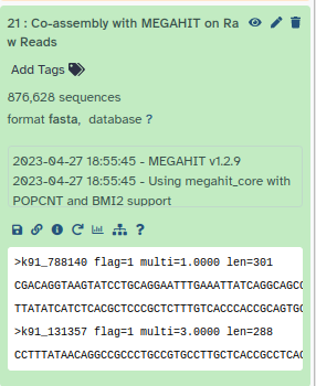
Co-assembly

Co-assembly with MEGAHIT

  1. MEGAHIT Tool with parameters
    • Select your input option: Paired-end collection
    • Run in batch mode?: Merge all fastq pair-end
    • Select a paired collection: Raw reads
    • Basic assembly options
      • K-mer specification method: Specify min, max, and step values
      • Minimum kmer size: 21
      • Maximum kmer size: 91
      • Increment of kmer size of each iteration: 12

Go Up


Co-assembly with MetaSPAdes

  1. MetaSPAdes Tool with following parameters
    • Pair-end reads input format: Paired-end: list of dataset pairs
      • FASTQ file(s): collection: Raw reads
    • Select k-mer detection option: User specific
      • K-mer size values: 21,33,55,77

NOTE! Slower than MEGAHIT

Go Up


Quality control of assembly

  1. Quast Tool with parameters
    • Assembly mode?: Individual assembly (1 contig file per samples)
      • Use customized names for the input files?: No, use dataset names
        • Contigs/scaffolds file: output MEGAHIT
      • Reads options: Illumina paired-end reads in paired collection (To make the job quicker, you can select Disabled here. The raw reads will then not been mapped to the assembly to compute metrics, like the coverage.)
        • FASTQ/FASTA files: Raw reads
    • Type of assembly: Metagenome
    • Output files: HTML report, PDF report, Tabular reports, Log file, Key metric summary (metagenome mode), Krona charts (metagenome mode without reference genomes)
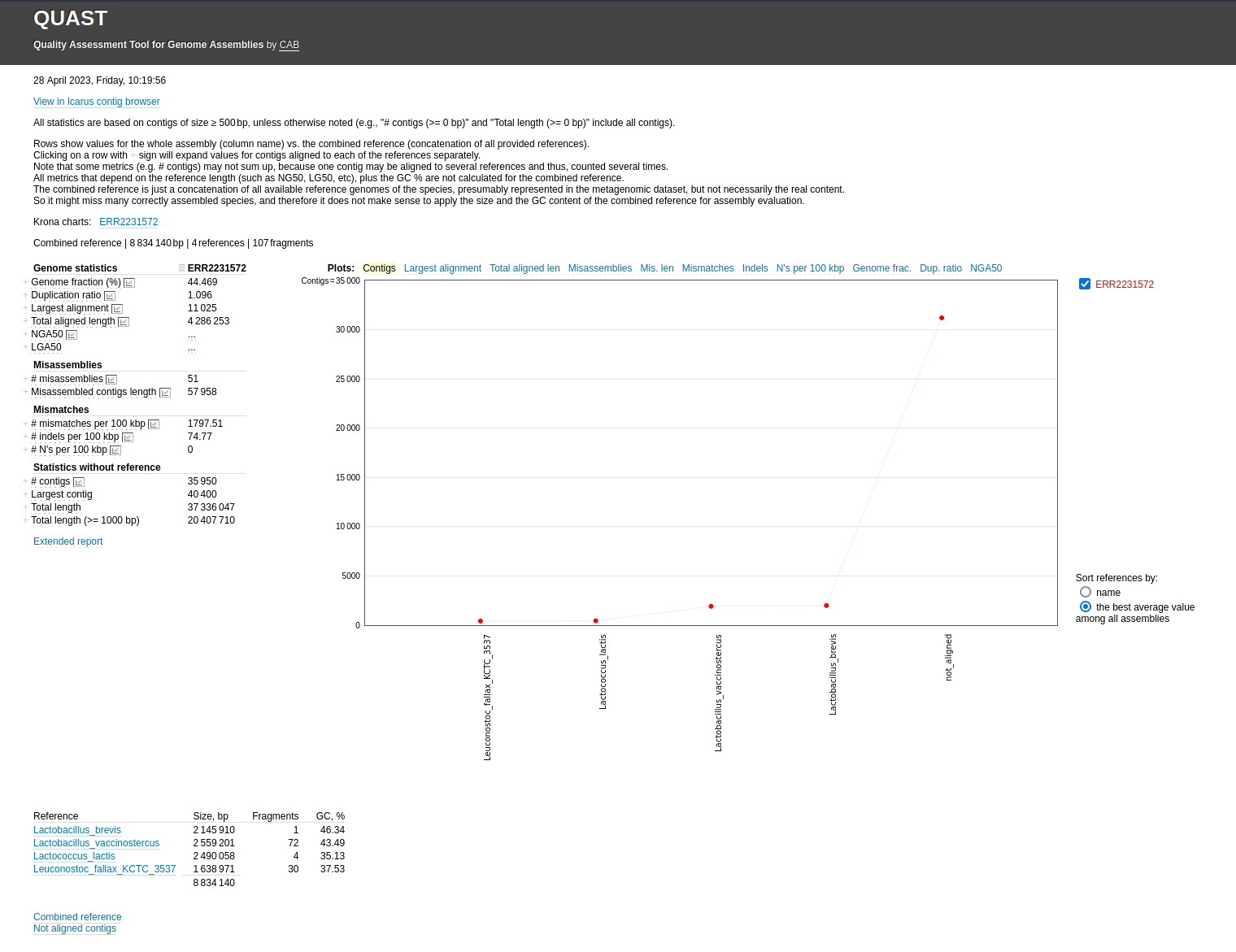
  2. Inspect the HTML reports

Go Up


Assembly statistics

See Quast Manual

  1. Genome statistics
    • Genome fraction (%): percentage of aligned bases in the reference genome

      Question

      • What is the genome fraction for ERR2231568? And for ERR2231572?
      • Which reference genome has the highest genome fraction for ERR2231568? And for ERR2231572?
    • Duplication ratio: total number of aligned bases / genome fraction * reference length

      Question

      • What is the duplication ratio for ERR2231568? And for ERR2231572?
      • Which reference genome has the highest duplication ratio for ERR2231568? And for ERR2231572?
  2. Read mapping: results of the mapping of the raw reads on the different assemblies (only if the Reads options is not disabled)
    • Alternative ways to compute coverage:
      • CoverM-CONTIG Tool with parameters:
        • Read type: Paired collection
        • One or more pairs of forward and reverse possibly gzipped FASTA/Q files for mapping in order: Raw Reads
      • Bowtie2 Tool with the following parameters:
        • Is this single or paired library: Paired-end Dataset Collection
        • FASTQ Paired Dataset: Raw reads
        • Will you select a reference genome from your history or use a built-in index?: Use a genome from the history and build index
        • Select reference genome: MEGAHIT output
        • Save the Bowtie2 mapping statistics to the history: Yes
  3. Misassemblies: joining sequences that should not be adjacent.
  4. Mismatches or mismatched bases in the contig-reference alignment
  5. Statistics without reference
    • # contigs: total number of contigs
    • Largest contig: length of the longest contig in the assembly
    • N50: length for which the collection of all contigs of that length or longer covers at least half an assembly

      N50 statistic defines assembly quality in terms of contiguity. If all contigs in an assembly are ordered by length, the N50 is the minimum length of contigs that contains 50% of the assembled bases. For example, an N50 of 10,000 bp means that 50% of the assembled bases are contained in contigs of at least 10,000 bp.

      When comparing N50 values from different assemblies, the assembly sizes must be the same size in order for N50 to be meaningful.

    • L50: number of contigs equal to or longer than N50

      In other words, L50 is the minimal number of contigs that cover half the assembly.

Go Up


Icarus contig browser

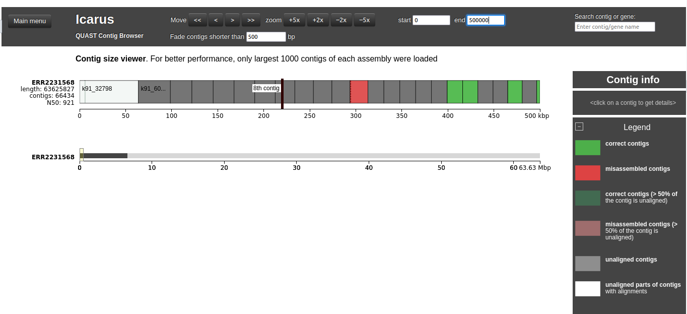
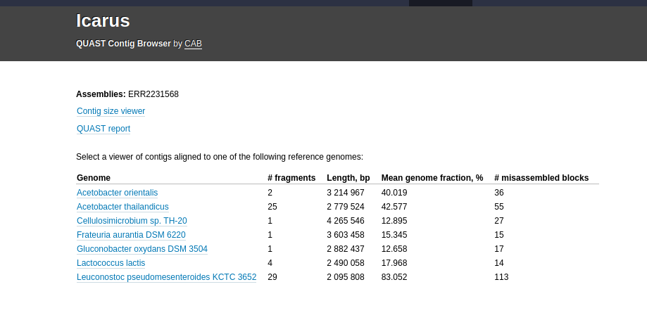
Icarus generates contig size viewer and one or more contig alignment viewers (if reference genome/genomes are provided) that are accessible from the HTML report, by clicking on View on Icarus contig browser.
Go Up


Contig size viewer

This viewer draws contigs ordered from longest to shortest. Let’s inspect this viewer for ERR2231568.

  1. Open the Contig size viewer for ERR2231568
  2. define start as 0 and end as 500000

Question

  1. What is the color of the first contig? Why?
  2. What is the red contig?

Solutions

  1. The first contig is white because >50% of the contigs is unaligned. By clicking on the contig, we see that only a small block is aligned:

    223.41 – 223.65 kbp to Leuconostoc_pseudomesenteroides_KCTC_3652_NZ_BMBP01000002.1.

  2. The red contig is a missamblied contig: it contains 2 blocks, with a translocation between them.

Click Main menu on the top left to go back to the main Icarus page.

Go Up


Contig alignment viewer

If a reference genome is provided, there should be a table on the main Icarus page that looks like:
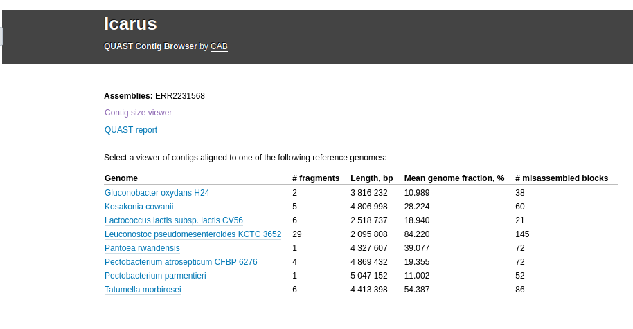
When clicking on the genome name, the contigs are displayed according to their mapping to the reference genome. The viewer can additionally visualize genes, operons, and read coverage distribution along the genome, if any of those were fed to QUAST.

  1. Open the Contig alignment viewer for ERR2231568 and Leuconostoc pseudomesenteroides KCTC 3652, the most covered by contigs

Question

  1. How are the organized the contigs on the top?
  2. What the different colors for the contigs?
  3. Why is there a big red block on the right?
  4. What is the graph on the bottom?

Solutions

  1. The contigs are displayed based on their mapping on the reference genome of Leuconostoc pseudomesenteroides KCTC 3652
  2. The different colors represent the different status for the contig: correct contigs, correct contigs but with >50% of the contig unaligned, misassembled blocks. unchecked misassembled blocks, ambiguously mapped contigs, alternative blocks of misassembled contigs, etc.
  3. The big red block on the right is contig k91_88833 with a misassembly on the left side, and overlap with 2 other contigs
  4. The graph on the bottom represents the GC percentage and coverage by contigs along the reference genome

Go Up


Identification of potential assembly error signature

VALET (VALidating mETagenomic assemblies) is a pipeline for performing de novo validation of metagenomic assemblies.

VALET checks a number of properties that should hold true for a correct assembly (e.g., mate-pairs are aligned at the correct distance from each other in the assembly, the depth of coverage is fairly uniform along contigs, etc.).

The violations of these invariants are reported allowing one to pinpoint areas that were potentially mis-assembled, or to compare the quality of different assemblies. For comparing multiple assemblies of the same data-sets, VALET also reports an overall estimate of the likelihood a particular assembly is correct.

  1. VALET Tool with paramaters:
    • Insert Candidate assemblies:
      • Candidate assembly file: contigs from metaSpades
      • Name of the assembly: spades
    • Insert Candidate assemblies:
      • Candidate assembly file: contigs from MEGAHIT
      • Name of the assembly: megahit
    • Type of input reads used for the assembly: Paired-collection
    • Input format: FASTQ
    • Assembly input reads: Raw Reads
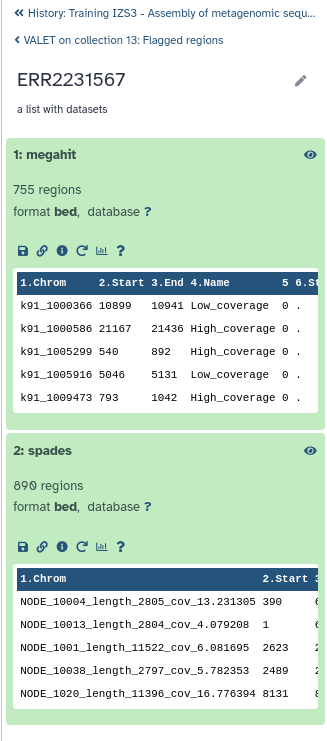
  2. Inspect the output files
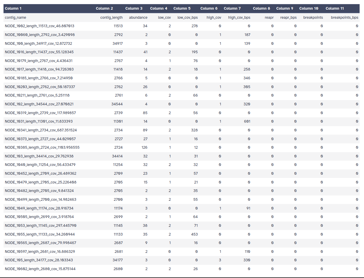
    • Summary: a breakdown of each contig’s number of misassemblies
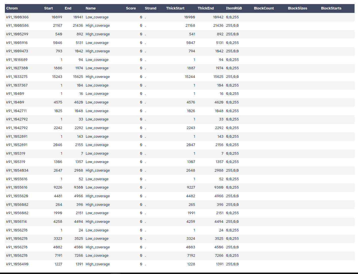
    • Flagged Regions: potential misassemblies
    • Suspicious Regions: Intersection of multiple misassembly signatures overlapping
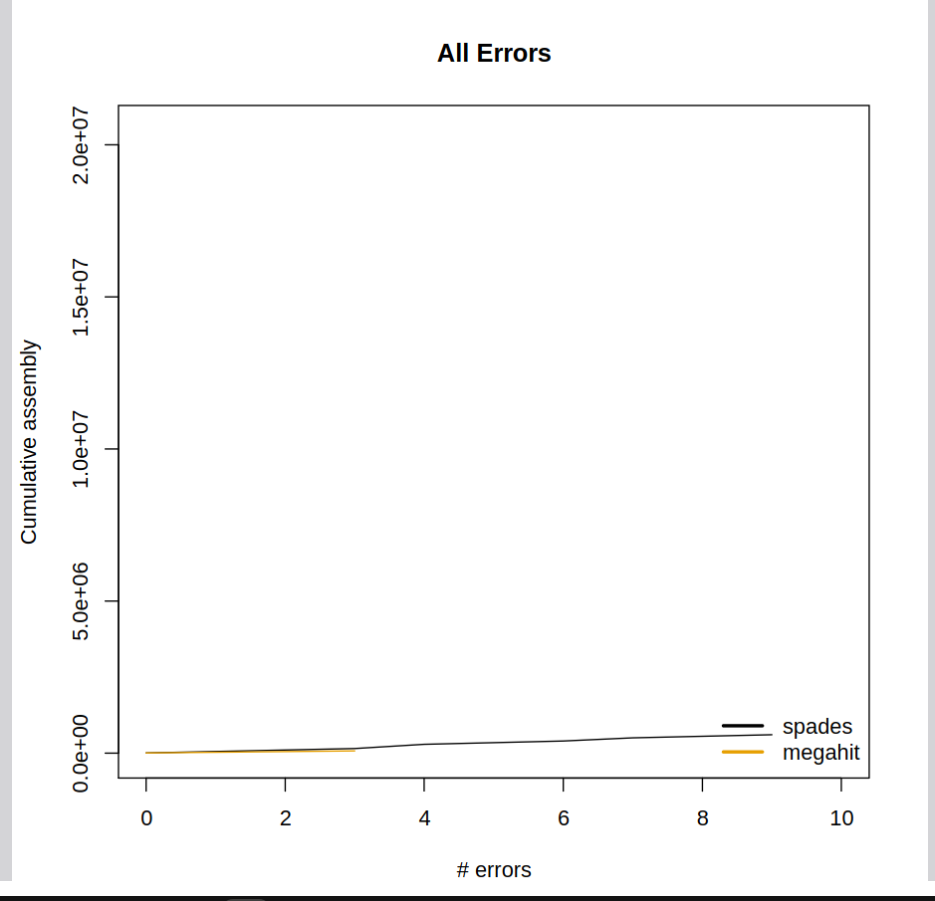
    • Comparison Plot: highlights the trade-off between contiguity and accuracy.

Go Up


Report Aggregation

  1. Run Bowtie2 on metaSpades output
  2. Run Bowtie2 on MEGAHIT output
  3. Run QUAST on metaSpades output
  4. Run QUAST on MEGAHIT output
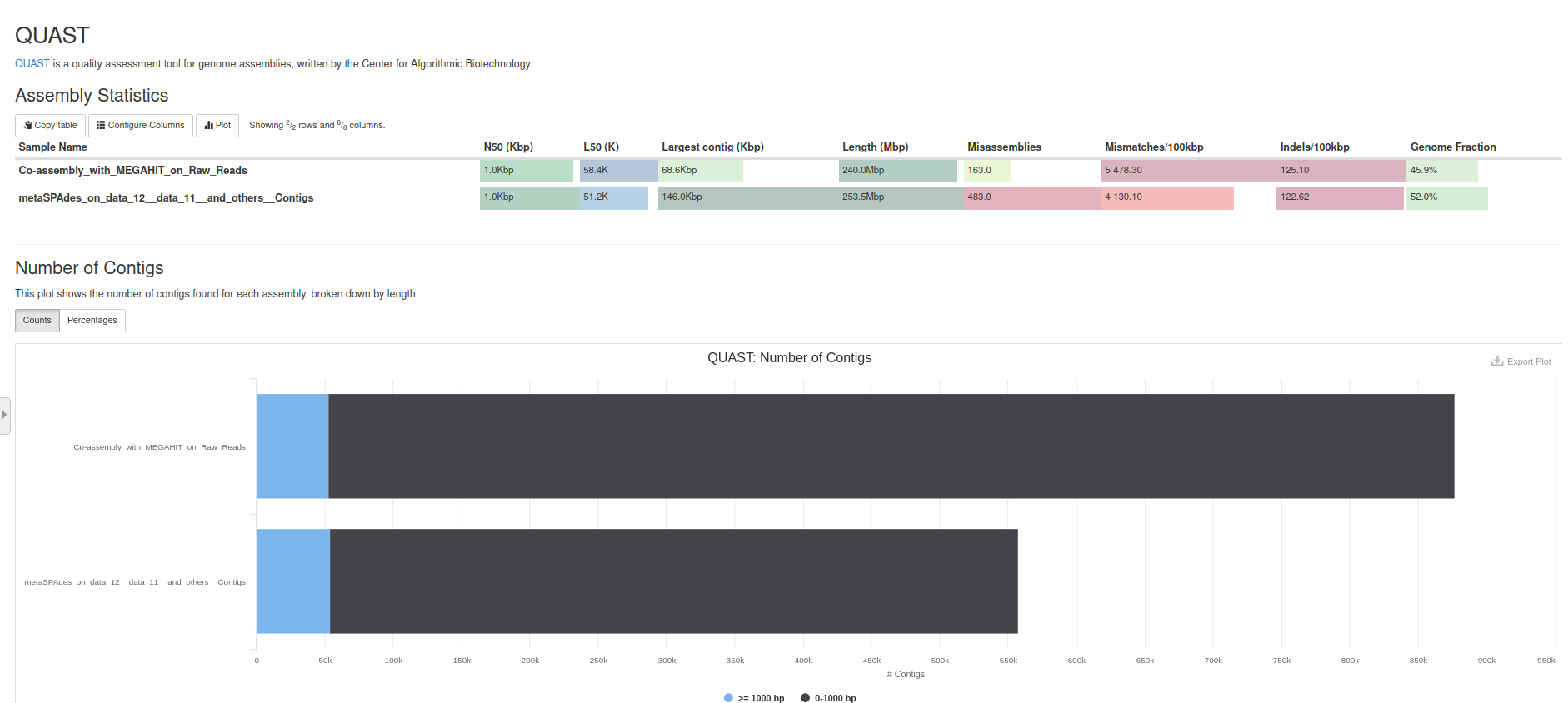
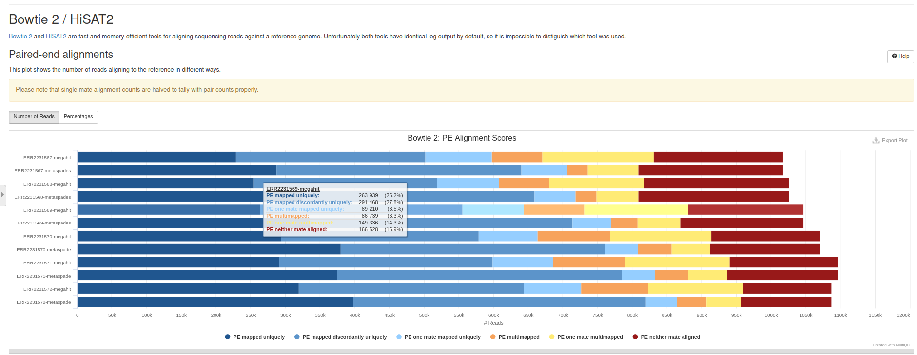
  5. MultiQC tool with following parameters
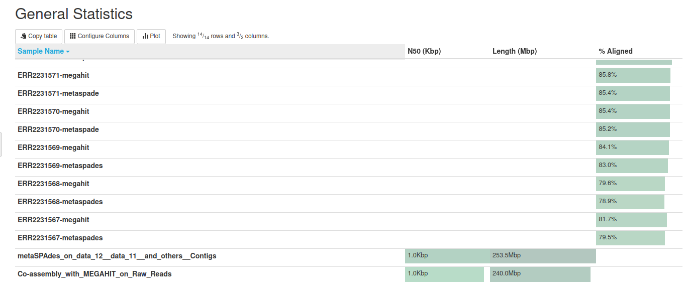
    • In “Results”:
    • Insert Results
      • Which tool was used generate logs?: QUAST
      • *In “QUAST Output”:
        • QUAST Output: QUAST Report on MEGAHIT
    • Insert Results
      • Which tool was used generate logs?: QUAST
      • *In “QUAST Output”:
        • QUAST Output: QUAST Report on metaSpades
    • Insert Results
      • Which tool was used generate logs?: Bowtie2
      • *In “Bowtie2 Output”:
        • Bowtie2 Output: Bowtie2 Mapping Stats on MEGAHIT
    • Insert Results
      • Which tool was used generate logs?: Bowtie2
      • *In “Bowtie2 Output”:
        • Bowtie2 Output: Bowtie2 Mapping Stats on metaSpades
        • Report title: Co-Assembly Report

General Statistics

QUAST

Bowtie2

Go Up


Conclusion

Metagenomic data can be assembled to, ideally, obtain the genomes of the species that are represented within the input data. But metagenomic assembly is complex and there are

  • different approaches like de Bruijn graphs methods
  • different strategies, such as co-assembly, when we assembly all samples together, and individual assembly, when we assembly samples one by one
  • different tools like MetaSPAdes and MEGAHIT

Go Up


Hands-On

Now, it’s your turn!

Go Up