Microbial Variant Calling
How do we detect differences between a set of reads from a microorganism and a reference genome?
Variant calling is the process of identifying differences between two genome samples.
Usually differences are limited to single nucleotide polymorphisms (SNPs)
and small insertions and deletions (indels).
Imagine that you have been asked to find the differences between a sample that has been sequenced and a known genome.
For example:
You have a new sample from a patient and you want to see if it has any differences from a well known reference genome  of the same species.

Typically, you would have a couple of fastq read files sent back to you from the sequencing provider and either an annotated or non annotated reference genome.
In this tutorial, we will use the tool Snippy
to find high confidence differences (indels or SNPs) between our known genome and our reads,
ie. finds SNPs between a haploid reference genome and your NGS sequence reads.
Snippy pipeline consists of 3 steps:
- Read mapping: to align the reads to the reference genome
BWA MEM with a custom set of settings which are very suitable to aligning reads for microbial type data
- Variant Calling: to decide (“call”) if any of the resulting discrepancies are real variants or technical artifacts that can be ignored
Freebayes with a custom set of settings
- Functional Effect Prediction: to describe what the predicted changes do in terms of the genes themselves.
SnpEff with a custom set of settings
The Galaxy wrapper for Snippy has the ability to change some of the underlying tool settings in the advanced section but it is not recommended.
Go Up
Get the data
The data is a subset of a real dataset from a Staphylococcus aureus bacteria.
We have a closed genome sequence and an annotation for our wildtype strain.
A whole-genome shotgun approach was used to produce a series of short sequence reads on an Illumina DNA sequencing instrument for the mutant strain.
- The reads are paired-end
- Each read is on average 150 bases
- The reads would cover the original wildtype genome to a depth of 19x
The files we will be using are:
- mutant_R1.fastq & mutant_R2.fastq - the read files in fastq format.
- wildtype.fna - The sequence of the reference strain in fasta format.
- wildtype.gbk - The reference strain with gene and other annotations in genbank format.
- wildtype.gff - The reference strain with gene and other annotations in gff3 format.
NOTE! This data is available at Zenodo
NOTE! Please, use
- Create a new history
- Upload datasets
https://zenodo.org/record/582600/files/mutant_R1.fastq
https://zenodo.org/record/582600/files/mutant_R2.fastq
https://zenodo.org/record/582600/files/wildtype.fna
https://zenodo.org/record/582600/files/wildtype.gbk
https://zenodo.org/record/582600/files/wildtype.gff
Go Up
Find variants with Snippy
We will now run the Snippy tool on our reads, comparing it to the reference.
Snippy is a tool for rapid bacterial SNP calling and core genome alignments.Snippy finds SNPs between a haploid reference genome and your NGS sequence reads. It will find both substitutions (snps) and insertions/deletions (indels).- If we give
Snippy an annotated reference, it will silently run SnpEff which will figure out the effect of any changes on the genes and other features.
- If we just give
Snippy the reference sequence alone without the annotations, it will not run SnpEff.
We have an annotated reference and so will use it in this case.
Snippy tool with the following parameters:
- Reference File: the wildtype.gbk file (if the genbank file is not selectable, make sure to change its datatype to ‘genbank’)
- Single or Paired-end reads: Paired
- Select first set of reads: mutant_R1.fastq
- Select second set of reads: mutant_R2.fastq
- Select all outputs
Go Up
Examine Snippy output
Snippy has taken the reads and:
- mapped them against the reference using
BWA MEM,
- looked through the resulting BAM file and found differences using some fancy Bayesian statistics (
Freebayes),
- filtered the differences for sensibility and finally checked what effect these differences will have on the predicted genes and other features in the genome.
It produces quite a bit of output, there can be up to 10 output files.

- snps vcf file: The final annotated variants in VCF format
- snps gff file: The variants in GFF3 format

- snps table: A simple tab-separated summary of all the variants

- snps summary: A summary of the SNPs called

- log file: A log file with the commands run and their outputs
- aligned fasta: A version of the reference but with - at position with depth=0 and N for 0 < depth < –mincov (does not have variants)
- consensus fasta: A version of the reference genome with all variants instantiated
- mapping depth: A table of the mapping depth
- mapped reads bam: A BAM file containing all of the mapped reads
- outdir: A tarball of the Snippy output directory for input into Snippy-core if required
Question
- Which types of variants have been found?
- What is the third variant called?
- What is the product of the mutation?
- What might be the result of such a mutation?
Go Up
View Snippy output in JBrowse
We could go through all of the variants like this and read them out of a text table,
but this is onerous and doesn’t really give the context of the changes very well.
In order to have a visualisation of the SNPs and the other relevant data, in Galaxy we can use JBrowse
JBrowse Tool with the following parameters
- Reference genome to display: Use a genome from history
- Select the reference genome: wildtype.fna
- Genetic Code: 11: The Bacterial, Archaeal and Plant Plastid Code
- In Track Group: sequence reads
- Insert Track Group
- Track Category: Gene Annotations
- Track Type: BAM Pileups
- BAM Track Data: bam file from
Snippy
- Autogenerate SNP Track: Yes
- Track Visibility: On for new users
- In Track Group: variants
- Insert Track Group
- Track Category: Variants
- Track Type: GFF/GFF3/BED Features
- GFF/GFF3/BED Track Data snps gff file from
Snippy
- Track Visibility: On for new users
- In Track Group:
- Insert Track Group
- Track Category:
- Track Type: GFF/GFF3/BED Features
- GFF/GFF3/BED Track Data: wildtype.gff
- JBrowse Track Type [Advanced]: Canvas Features
- Click on JBrowse Styling Options [Advanced]
- JBrowse style.label: product
- JBrowse style.description product
- Track Visibility: On for new users
Go Up
Inspecting the SNPs using JBrowse
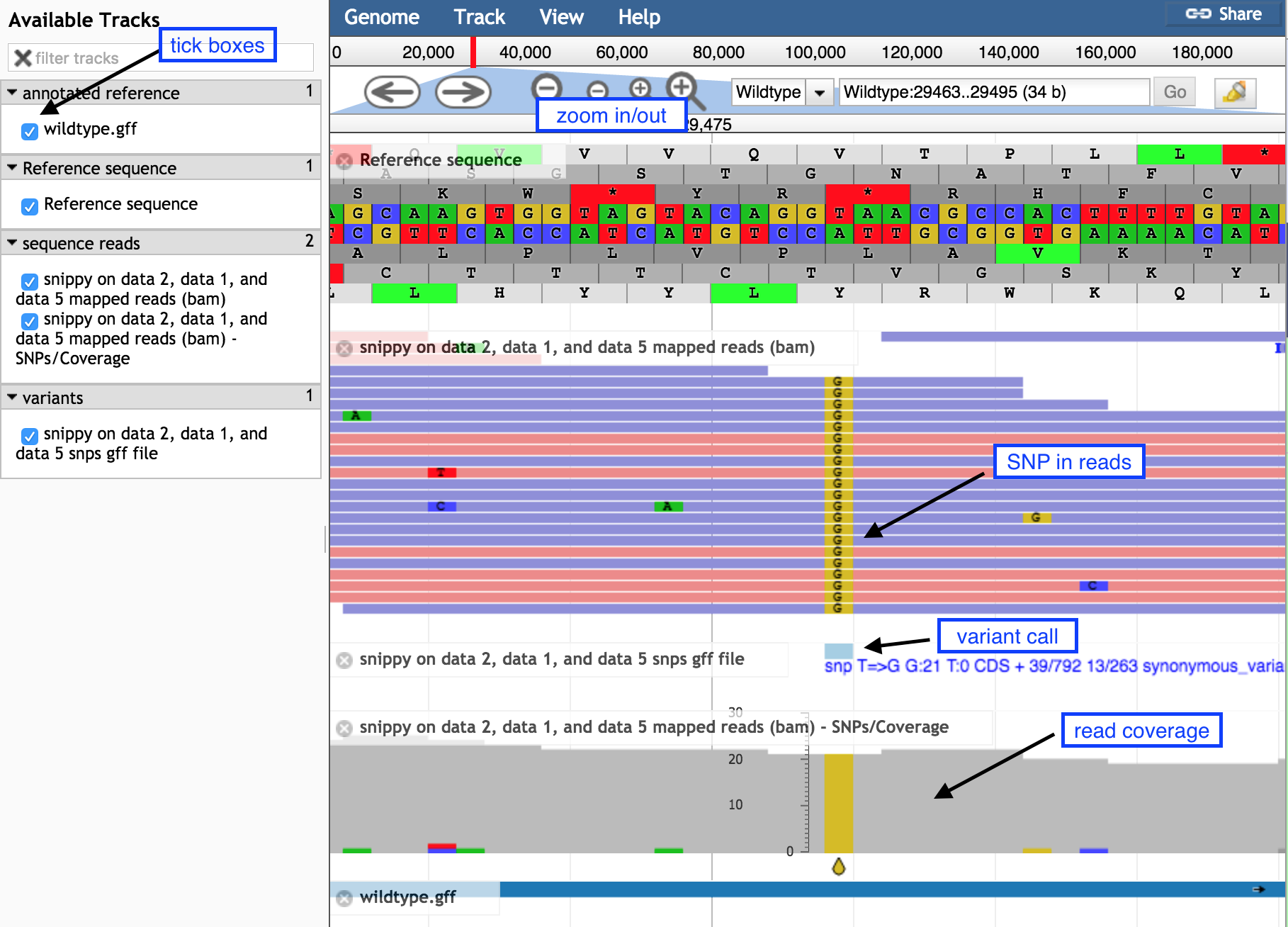
- Display all the tracks and practice maneuvering around
- Click on the tick boxes on the left to display the tracks
- Zoom out by clicking on the
minus button to see sequence reads and their coverage (the grey graph)
- Zoom in by clicking on the
plus button to see
- probable real variants (a whole column of SNPs)
- probable errors (single one here and there)

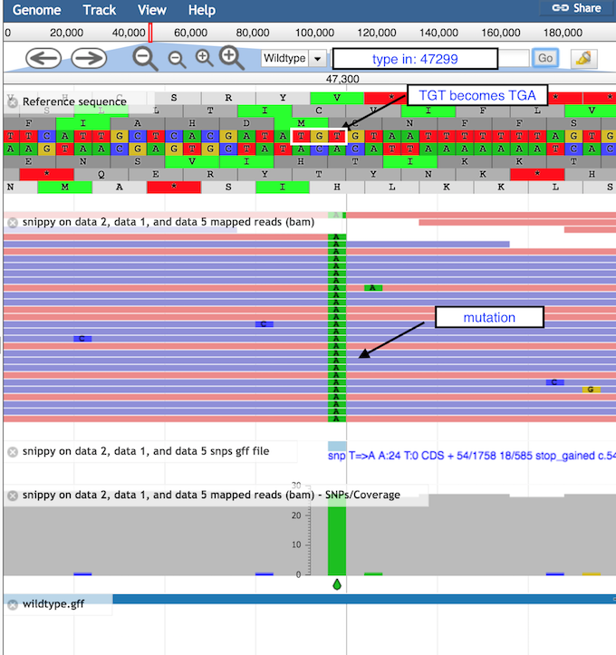
- Look at the stop SNP
- Type 47299 in the coordinates box
- Click on Go to see the position of the SNP discussed above

Question
- What is the correct codon at this position?
- What is the mutation found here?
Go Up
Conclusion
By running a tool such as Snippy on your read files and reference genome,
we can find where the biologically important changes between genomes
of different strains occur and perhaps what they mean to the phenotype
- We used a tool called
Snippy to call variants between our reads and our reference genome.
- As our reference genome had annotations, we could see what effect the changes have on the features as annotated in the reference and therefore make inferences on the possible changes to the phenotype.
- We used the
JBrowse genome browser to visualise what these changes look like
Go Up
Hands-On
Now, it’s your turn!
Go Up


