Annotation and exploration of a draft bacterial genome, including gene prediction, identification of genomic components, evaluation of annotation results, and visualization of annotated features.
After sequencing and assembly, a genome can be annotated. It is an essential step to describe the genome.
Genome annotation consists in describing the structure and function of the components of the genome, by predicting, analyzing, and interpreting them in order to extract their biological significance and understand the biological processes in which they participate.
Among other things, it identifies the locations of genes and all the coding regions in a genome (structural annotation) and determines what those genes do (functional annotation).
To illustrate the process to annotate a bacterial genome, we take the assembly generated in the previous tutorial.
Before starting the analysis, prepare your Galaxy workspace as follows:
Create a new Galaxy history and give it a meaningful name.
Import the Shovill contigs dataset into the new history by dragging and dropping it from a previous history (see here for instructions on managing and copying datasets between histories).
For annotating the contigs, several tools can be used for this purpose, including Prokka and Bakta.
BaktaBakta is a tool for rapid and standardized annotation of bacterial genomes and plasmids from both isolates and metagenome-assembled genomes (MAGs).
Bakta with the following parameters:
Bakta can generate many outputs. Here we selected:
annotation_and_sequences in GFF3
A GFF is a tab delimited file with 9 fields per line:
seqid: The name of the sequence where the feature is located.
source: The algorithm or procedure that generated the feature. This is typically the name of a software or database.
type: The feature type name, like “gene” or “exon”. In a well structured GFF file, all the children features always follow their parents in a single block (so all exons of a transcript are put after their parent “transcript” feature line and before any other parent transcript line). In GFF3, all features and their relationships should be compatible with the standards released by the Sequence Ontology Project.
start: Genomic start of the feature, with a 1-base offset. This is in contrast with other 0-offset half-open sequence formats, like BED.
end: Genomic end of the feature, with a 1-base offset. This is the same end coordinate as it is in 0-offset half-open sequence formats, like BED.
score: Numeric value that generally indicates the confidence of the source in the annotated feature. A value of “.” (a dot) is used to define a null value.
strand: Single character that indicates the strand of the feature. This can be “+” (positive, or 5’->3’), “-“, (negative, or 3’->5’), “.” (undetermined), or “?” for features with relevant but unknown strands.
phase: phase of CDS features; it can be either one of 0, 1, 2 (for CDS features) or “.” (for everything else). See the section below for a detailed explanation.
attributes: A list of tag-value pairs separated by a semicolon with additional information about the feature.
summary with annotations as simple human readable TSV
This a table with 9 columns (Sequence Id, Type, Start, Stop, Strand, Locus Tag, Gene, Product, DbXrefs).
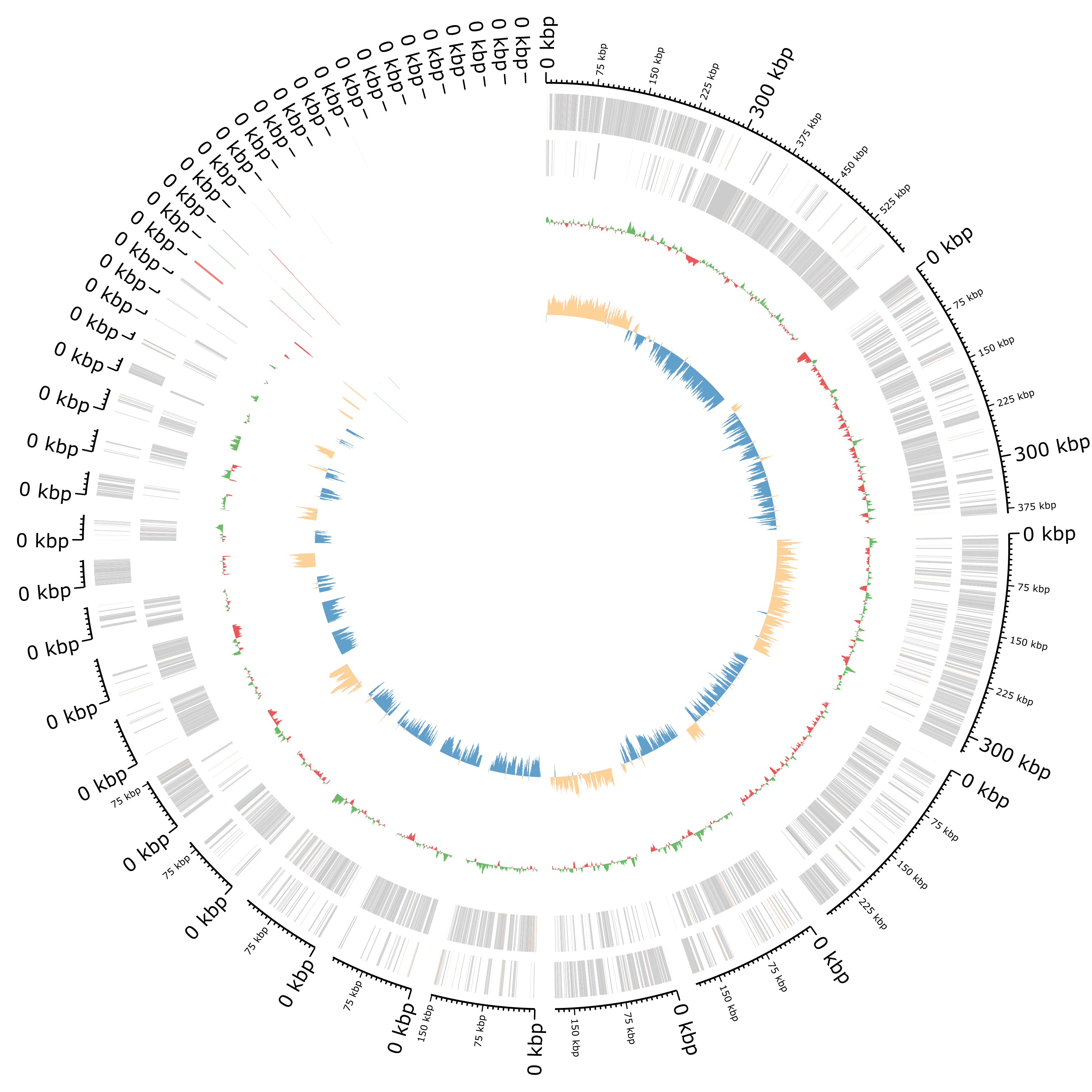
Plot of the annotation as circular genome annotation
Question
ProkkaProkka is a wrapper: it collects together several pieces of software
(from various authors), and so avoids “re-inventing the wheel”.
Prokka finds and annotates features (both protein coding regions and RNA genes, i.e. tRNA, rRNA)
present on a sequence, using a two-step process for the annotation of protein coding regions:
protein coding regions on the genome are identified using Prodigal;
the function of the encoded protein is predicted by similarity to proteins in one of many protein or protein domain databases.
Prokka is a software tool that can be used to annotate bacterial, archaeal and viral genomes quickly,
generating standard output files in GenBank, EMBL and gff formats.
Prokka Tool with the following parameters (leave everything else unchanged):
Once Prokka has finished, examine each of its output files.
| Extension | Description |
|---|---|
| .gff | This is the master annotation in GFF3 format, containing both sequences and annotations. It can be viewed directly in Artemis or IGV. |
| .gbk | This is a standard Genbank file derived from the master .gff. If the input to prokka was a multi-FASTA, then this will be a multi-Genbank, with one record for each sequence. |
| .fna | Nucleotide FASTA file of the input contig sequences. |
| .faa | Protein FASTA file of the translated CDS sequences. |
| .ffn | Nucleotide FASTA file of all the prediction transcripts (CDS, rRNA, tRNA, tmRNA, misc_RNA) |
| .sqn | An ASN1 format “Sequin” file for submission to Genbank. It needs to be edited to set the correct taxonomy, authors, related publication etc. |
| .fsa | Nucleotide FASTA file of the input contig sequences, used by “tbl2asn” to create the .sqn file. It is mostly the same as the .fna file, but with extra Sequin tags in the sequence description lines. |
| .tbl | Feature Table file, used by “tbl2asn” to create the .sqn file. |
| .err | Unacceptable annotations - the NCBI discrepancy report. |
| .log | Contains all the output that Prokka produced during its run. This is a record of what settings you used, even if the –quiet option was enabled. |
| .txt | Statistics relating to the annotated features found. |
| .tsv | Tab-separated file of all features: locus_tag,ftype,len_bp,gene,EC_number,COG,product |
Bakta gives a lot of information already, especially regarding CDSs or RNAs,
but some structural annotation might be missing, e.g. plasmids, or interesting to identify independently.
In assembled bacterial genomes, plasmids often appear as separate contigs, distinct from the chromosomal sequence.
For this reason, dedicated tools are commonly used to identify plasmid-derived contigs and distinguish
plasmid-associated genes from chromosomal genes,
a distinction that is particularly important
for antimicrobial resistance (AMR) analyses.
To identify plasmids in our contigs, we use PlasmidFinder, a tool for the identification and typing of plasmid sequences in Whole-Genome Sequencing. It uses the plasmidfinder database with hundreds of sequences to predict the plasmid in the data.
PlasmidFinder with the following parameters:
PlasmidFinder generates several outputs:
raw_results.txt: A text file containing the result table and alignments
results.tsv: A tabular file with the following columns:
Database
Plasmid: Plasmid against which the input genome has been aligned.
Identity: Percent identity in the alignment between the best matching plasmid in the database and the corresponding sequence in the inputgenome (also called the high-scoring segment pair (HSP)). A perfect alignment is 100%, but must also cover the entire length of the plasmid in the database (compare example 1 and 3).
Query/Template Length: Query length is the length of the best matching plasmid in the database, while HSP length is the length of the alignment between the best matching plasmid and the corresponding sequence in the genome (also called the high-scoring segment pair (HSP)).
Contig: Name of contig the plasmid is found in.
Position in contig: Starting position of the found gene in the contig.
Note: Notes about the plasmid
Accession number: Reference Genbank accession number accoding to NCBI for the plasmid in the database.
plasmid.fasta: A fasta file containing the best matching sequences from the query genome
hit_in_genome.fasta: A fasta file containing the best matching plasmid genes from the database
Question
How many plasmid sequences have been found?
Where are they located?
Are these sequences all associated with Staphylococcus aureus? (Looking at the accession number on the NCBI)
What can we conclude about contig00019?
Integrons are genetic mechanisms that allow bacteria to adapt and evolve rapidly through the stockpiling and expression of new genes. An integron is minimally composed of:
a gene encoding for a site-specific recombinase (intI)
a proximal recombination site (attI), which is recognized by the integrase and at which gene cassettes may be inserted
a promoter (Pc) which directs transcription of cassette-encoded genes
To detect integrons, we will use IntegronFinder
IntegronFinder with the following parameters:
IntegronFinder generates 2 outputs:
A summary with for each sequence in the input the number of identified CALIN elements, In0 elements, and complete integrons.
An integron annotation file as a tabular
Question
Insertion sequence (IS) element is a short DNA sequence that acts as a simple transposable element. IS are the smallest but most abundant autonomous transposable elements in bacterial genomes. They only code for proteins implicated in the transposition activity. They play then a key role in bacterial genome organization and evolution.
To detect IS elements, we will use ISEScan.
ISEScan with the following parameters:
ISEScan generates several files:
A summary as a table
The results as a table
The results as a GFF file
Several FASTA files:
Question
How many IS elements have been detected?
Where are they located?
What the different IS families?
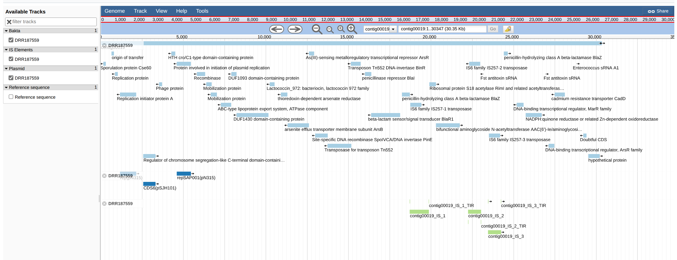
We would like to look at the annotation using JBrowse with several information:
Annotations identified by Bakta
Plasmid sequences identified by PlasmidFinder
Integrons identified by IntegronFinder
IS elements identified by ISEscan
JBrowse needs the annotations to be in GFF format.
Bakta and ISEscan generated both GFF files.
For PlasmidFinder and IntegronFinder, we need to format the outputs.
PlasmidFinder generated the results.tsv with all needed information. To transform it to a GFF, we need to:
Split the 6th column on .. to have start and end into 2 separated columns
Remove in the content of column 5 what is after the contig name
Remove the 1st line
Transform to GFF3
Replace Text in a specific column with the following parameters:
n column: Column: 6
Find pattern: (.)..(.)
Replace with: \1\t\2
This will split the content of the 6th column on .. and put it into column 6 and column 7. Column 7 will be then replaced.
n column: Column: 5
Find pattern: (.)( len.)
Replace with: \1
This will remove in the content of column 5 what is after the contig name
Select last lines from a dataset (tail) with the following parameters:
Text file: output of Replace Text above
Operation: Keep everything from this line on
Number of lines: 2
Table to GFF3 with the following parameters:
Table: output of the above Select last tool step
Source column or value: 1
IntegronFinder tabular output can be transformed to GFF by:
Replace NA values on column 7 by 0
Remove the first two lines
Transform to GFF3
Replace Text in a specific column with the following parameters:
n column: Column: 7
Find pattern: NA
Replace with: 0
Select last lines from a dataset (tail) with the following parameters:
Text file: output of Replace Text above
Operation: Keep everything from this line on
Number of lines: 3
Table to GFF3 with the following parameters:
Table: output of the above Select last tool step
Source column or value: IntegronFinder
We can now launch JBrowse with different information track.
JBrowse with the following parameters:
Bakta)ISEScan
- JBrowse Track Type [Advanced]: Neat Canvas Features
- Track Visibility: On for new usersIf integrons are found as IntegronFinder
JBrowseIn the output of the JBrowse you can view the genes, IS, plasmid, etc on the contigs.
With the search tools you can easily find genes of interest.
JBrowse can handle many inputs and can be very useful.
Question
Have all sequences identified by PlasmidFinder on contig19 been identified by Bakta?
Have all sequences identified by ISEScan on contig19 been identified by Bakta?
In this tutorial, contigs were annotated with different tools and then visualized.