From raw reads to insights: A hands-on guide to bacterial genomics
You have mastered the theory and practiced with curated demo datasets.
Today, we step out of the tutorial zone.
This session is about real data.
Real-world sequencing is messy, unpredictable, and rarely perfect.
You are no longer here to just follow commands —
you are here to practice the decision-making process required to transform raw,
noisy reads into a scientifically robust genome assembly.
In this hands-on exercise we will analyze a small collection of Serratia marcescens isolates.
The main questions we aim to answer are:
Raw reads
│
▼
Quality Control (Falco → MultiQC → fastp)
│
▼
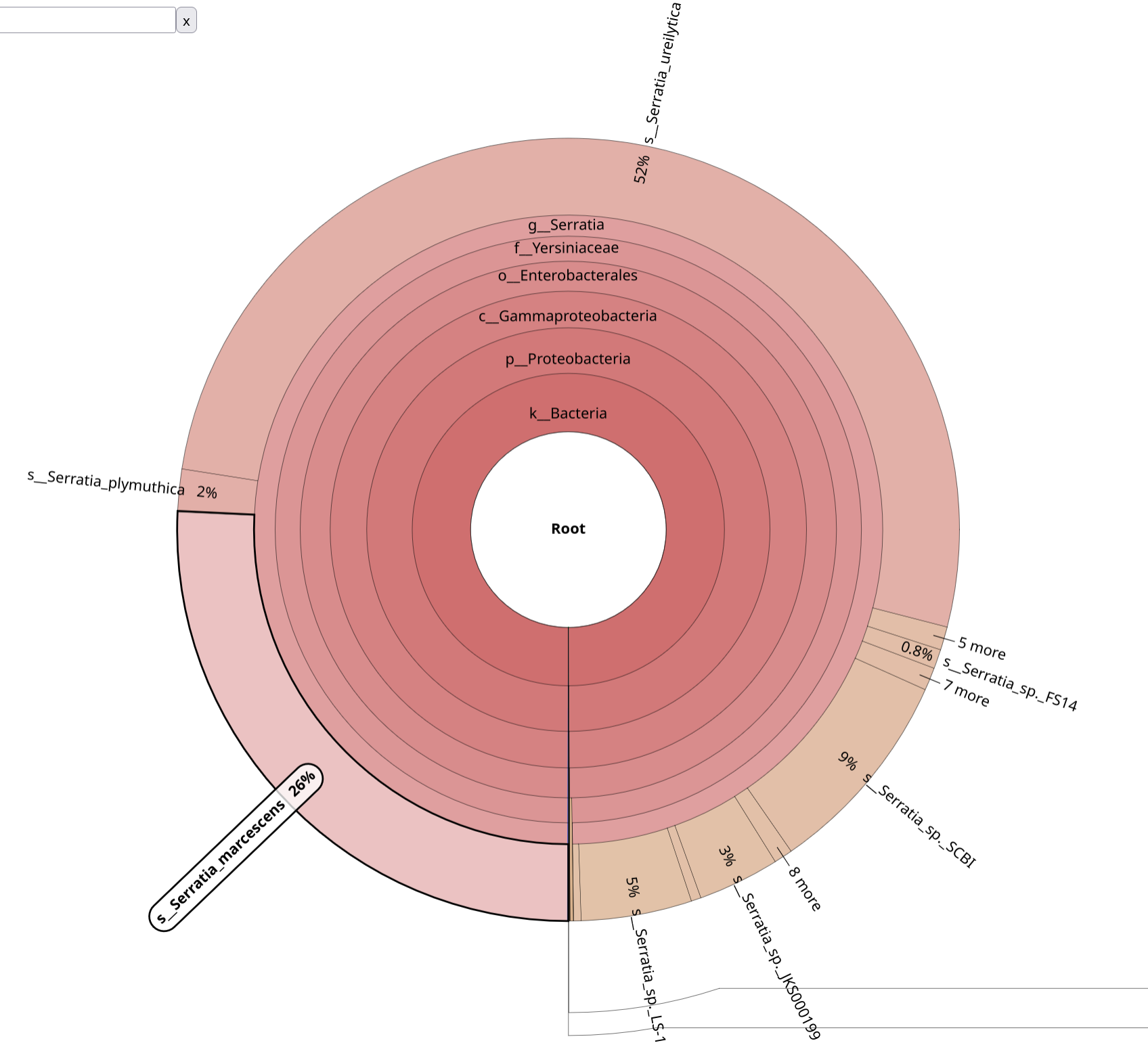
Contamination detection (Kraken2 → Bracken → Krona)
│
▼
Genome assembly (Shovill)
│
▼
Assembly assessment (QUAST → MultiQC)
│
▼
Genome annotation (Bakta)
│
▼
Functional profiling (StarAMR, ABRicate)
│
▼
Comparative genomics (Roary pangenome)
│
├── Accessory genome tree
├── Core genome phylogeny
└── SNP phylogeny (Snippy)
│
▼
Species confirmation (FastANI)
|
▼
Population structure (PopPUNK)
To eliminate local installation bottlenecks, we will use the public Galaxy instances:
We will work with a dataset pre-loaded into a shared Galaxy history.
Click Import.
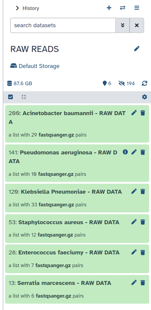
+ icon).Serratia Analysis).At this stage, you are ready to begin the analysis pipeline.
Before trimming or assembling anything, always inspect your data.
See the dedicated tutorial section: Quality Control
Falco Tool with the following parameters
MultiQC on Falco RawData
fastp with the following parameters:
Rename fastp output as Filtered Reads
MultiQC on the JSON output generated by fastpBefore moving to next step, confirm:
If all criteria are met → proceed to next step.
Otherwise → adjust trimming parameters and repeat QC.
When sequencing a genome, contamination from foreign organisms may be inadvertently mixed with the genomic material of the species of interest.
For this reason, when working with bacterial isolates, it is crucial to:
Confirming species identity and detecting contamination are essential to ensure the accuracy and reliability of the analysis, and to prevent misleading results that could compromise downstream interpretation (assembly quality, annotation, AMR detection, phylogenetic analysis).
For detailed instructions, interpretation guidelines, and tool configuration, please refer to the dedicated tutorial section: Checking expected species and contamination in bacterial isolate
Kraken2 Tool with the following parameters:
Bracken Tool with the following parameters:
Krakentools: Convert kraken report file Tool with the following parameters:
BrackenKrona pie chart Tool with the following parameters:
Krakentools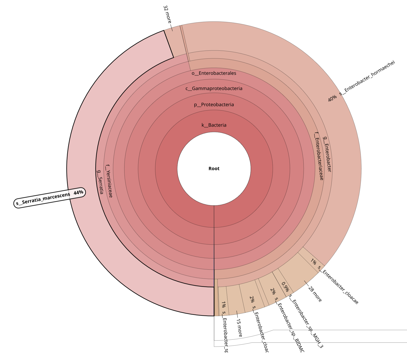
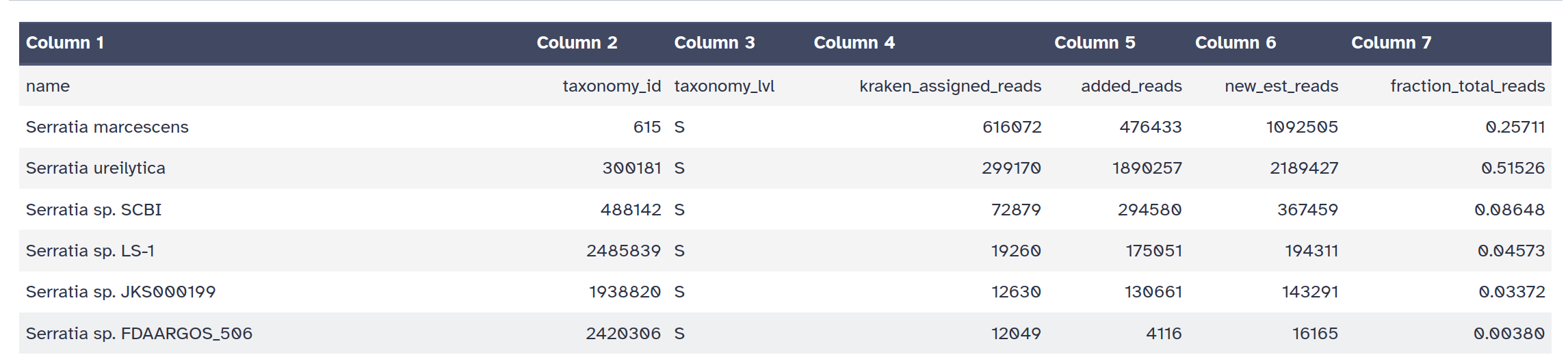
Before proceeding to assembly, confirm:
If criteria are met → proceed to assembly.
Otherwise → investigate contamination before continuing or remove dirty dataset
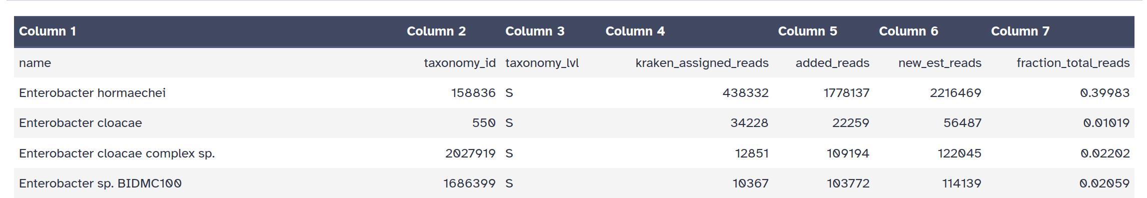
From the taxonomic profiling results, samples 044 and 046 show clear evidence
of contamination and do not meet the criteria defined in the contamination checklist.
These two datasets must therefore be excluded from downstream analysis.
Remove 044 and 046 from the collection.
We will proceed with de novo assembly using the remaining four clean datasets.
For educational purposes, we will intentionally create three scenarios:
044, 046)044The objective is to evaluate how contamination propagates through the pipeline and impacts assembly quality and downstream interpretation.
After quality control and contamination filtering, we are ready to reconstruct the genome.
De novo assembly aims to rebuild the bacterial genome from short sequencing reads without relying on a reference sequence.
For a detailed explanation please refer to the dedicated tutorial section: Genome Assembly of a bacterial genome
Shovill with the following parameters:
--isolateRename output as CONTIGS
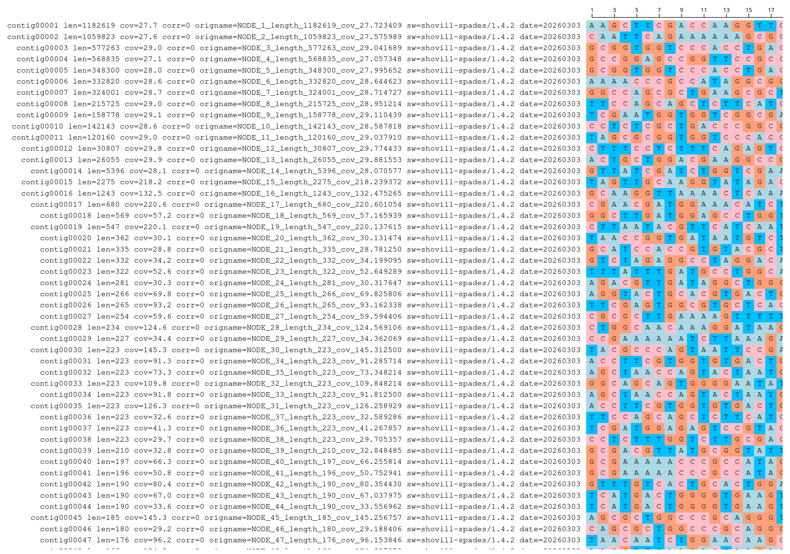
Click on the title of your file to see the row of small icons for saving, linking etc:
![]()
Click on the visualise icon and then select the Multiple Sequence Alignment tool. You should see something like this:
Quast Tool with parameters
ShovillMultiQC tool with following parameters
QUASTQUAST Report on Shovill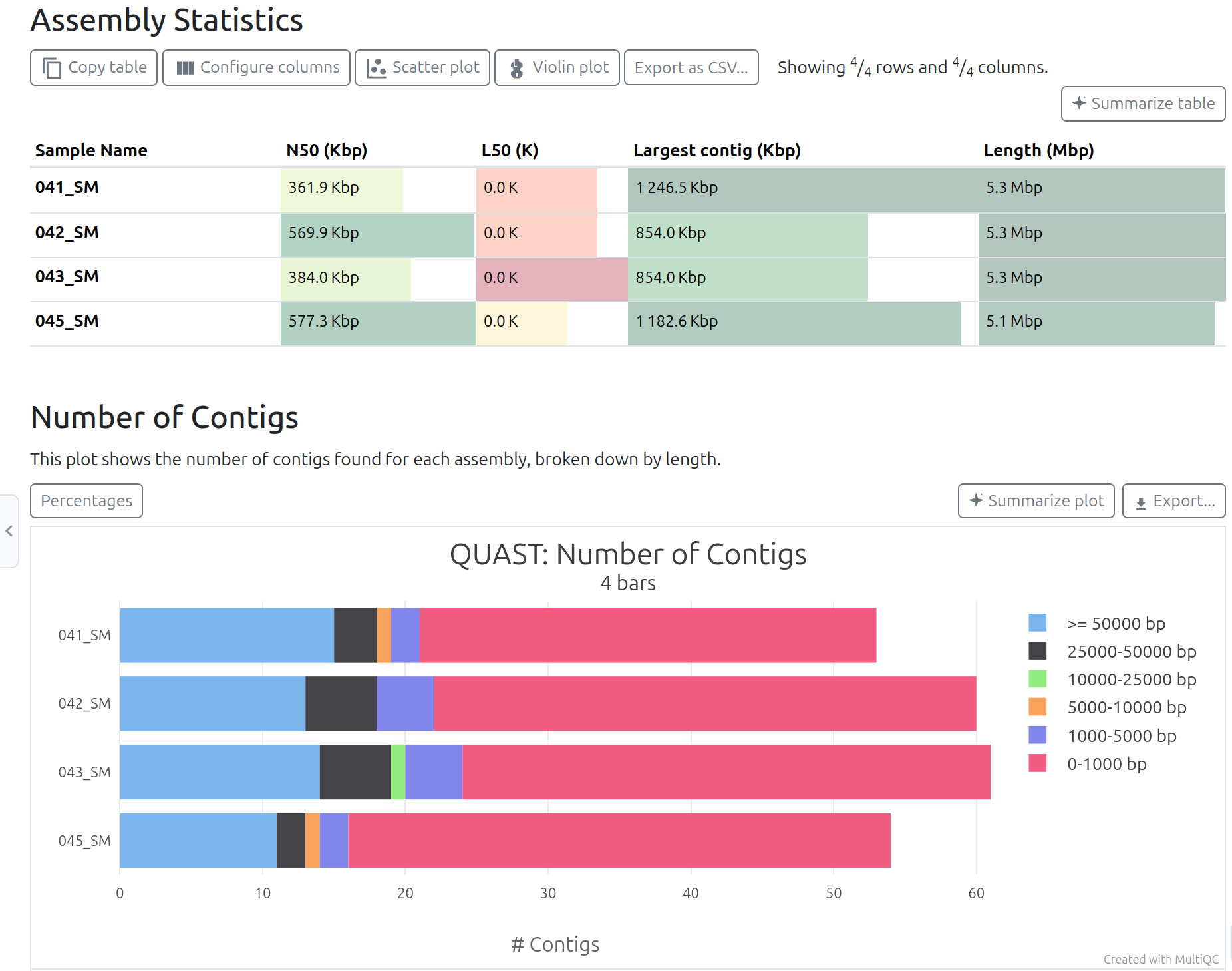
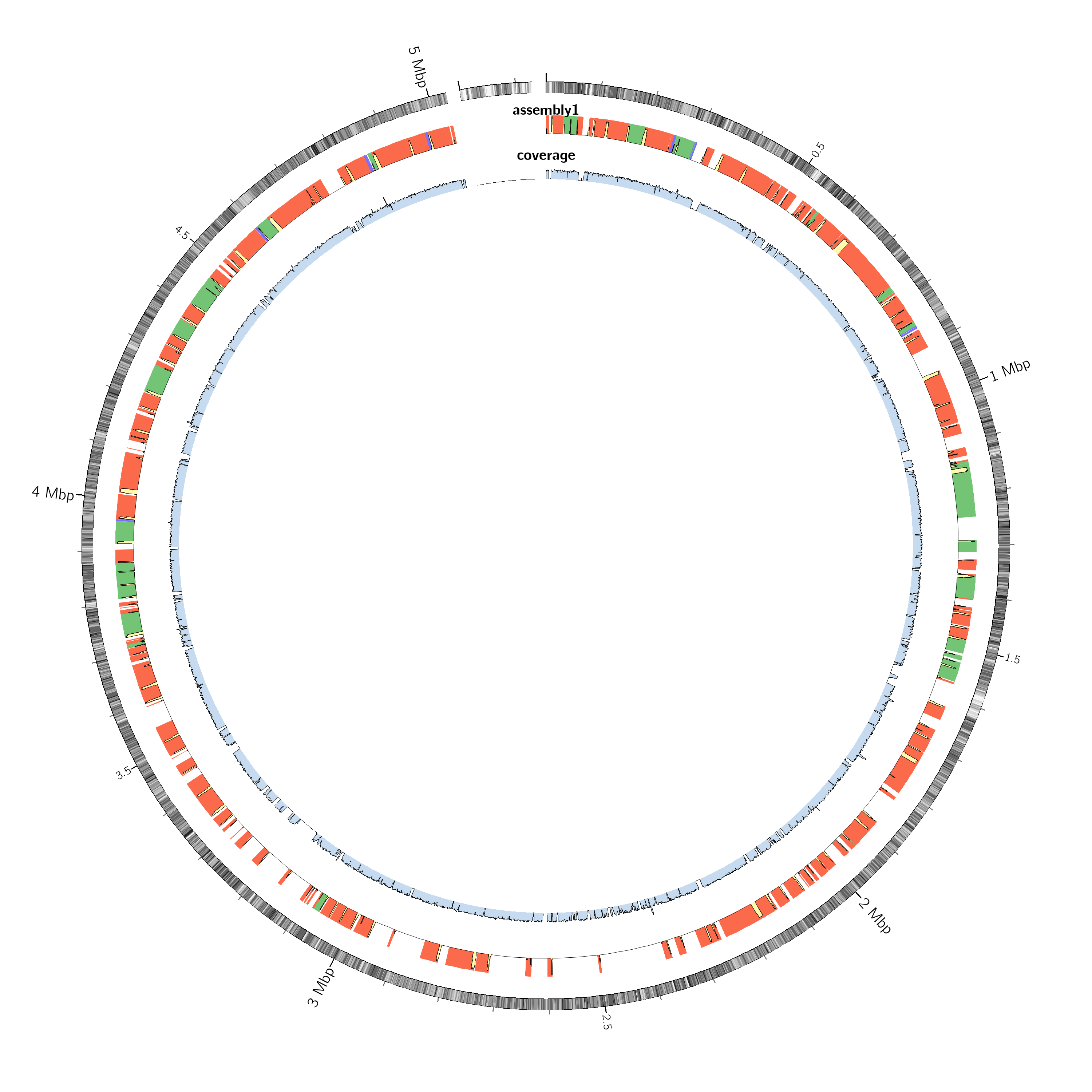
When a suitable reference genome is available, QUAST can also be run in reference-based mode.
In this case, the assembled contigs are aligned to the reference genome, allowing additional metrics to be calculated.
This analysis provides information such as:
QUAST can also generate a Circos plot showing how the assembled contigs align to the reference genome.
In this plot:
This visualization helps identify:
After running Shovill, evaluate your assembly using the following key metrics
(e.g. from QUAST OT MultiQC output).
If all criteria are satisfied → assembly is technically sound.
If one or more major criteria fail →
reconsider contamination, read quality, or sequencing depth.
After verifying that the assembly meets quality standards, we proceed to genome annotation.
Genome annotation aims to:
For detailed explanation, please refer to the dedicated tutorial: Bacterial Genome Annotation
Bakta with the following parameters:
MultiQC tool with following parameters
BaktaBakta Summary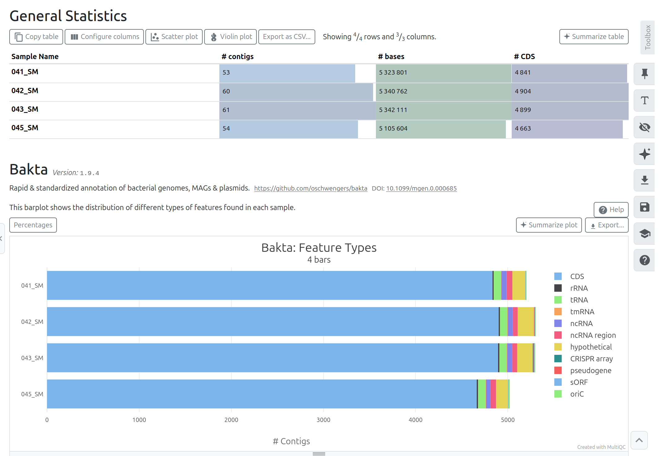
After completion, verify:
Large discrepancies in gene count or missing core features (e.g., rRNA genes) may indicate:
If annotation metrics are coherent → proceed to downstream analysis.
Beyond core genome annotation, additional mobile genetic elements can be explored. These analyses are interpretative and must be evaluated critically.
Plasmid detection is exploratory.
Integron detection is exploratory.
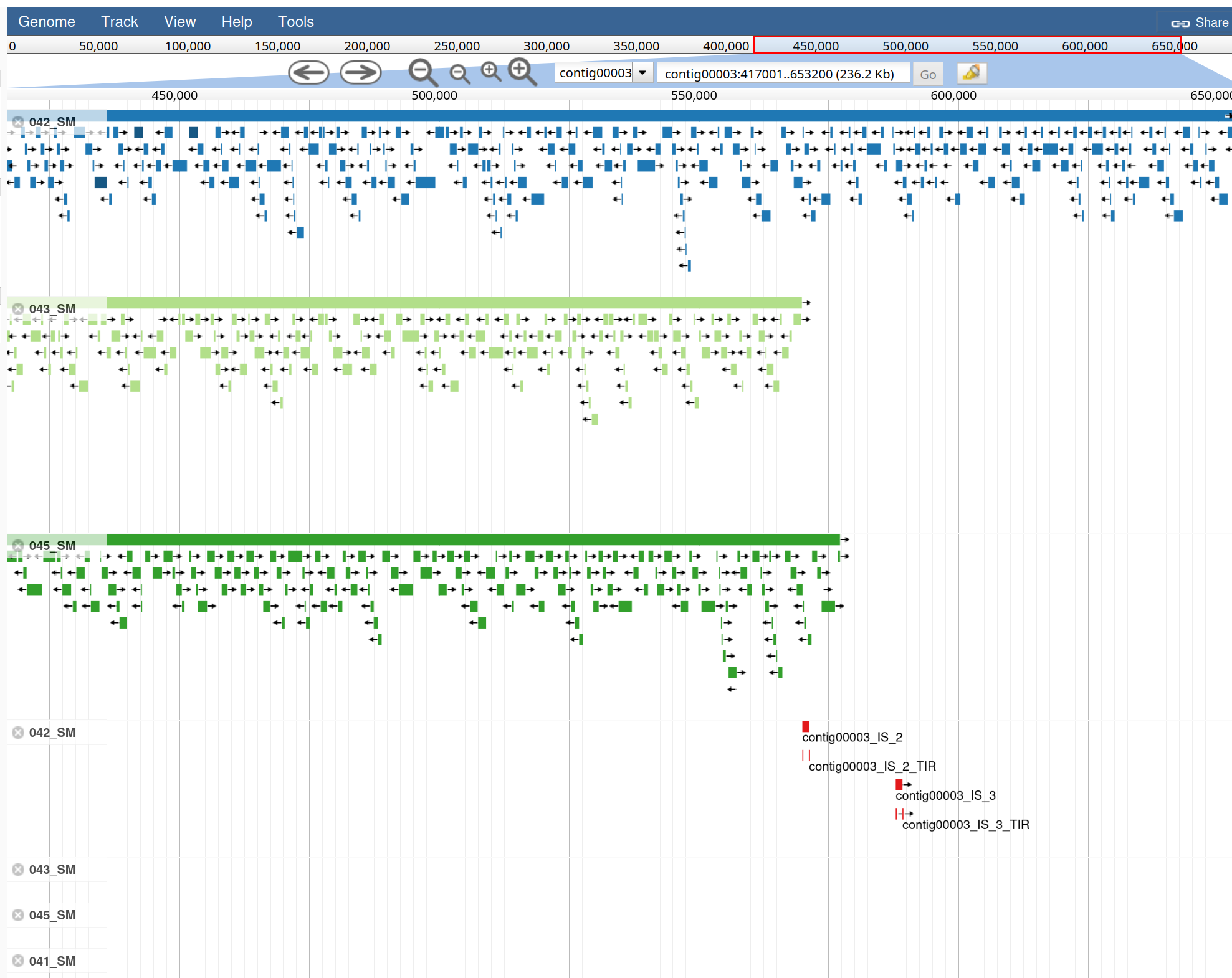
Insertion Sequences (IS) detection is exploratory.
In our dataset:
Interpretation:
We can now launch JBrowse with different information track.
JBrowse with the following parameters:
Bakta)ISEScanIf integrons are found as IntegronFinder
After genome annotation, additional analyses can be performed to explore clinically relevant genomic features.
In this section we will investigate:
AMR detection allows us to identify genes that may confer resistance to antibiotics, while virulence factor analysis helps reveal genetic determinants involved in pathogenicity, such as toxins, adhesion systems, secretion systems, and iron acquisition mechanisms.
These analyses provide insight into the potential clinical relevance and pathogenic profile of the organism.
For detailed explanations of the methodologies, databases, and interpretation of results, please refer to the dedicated tutorials:
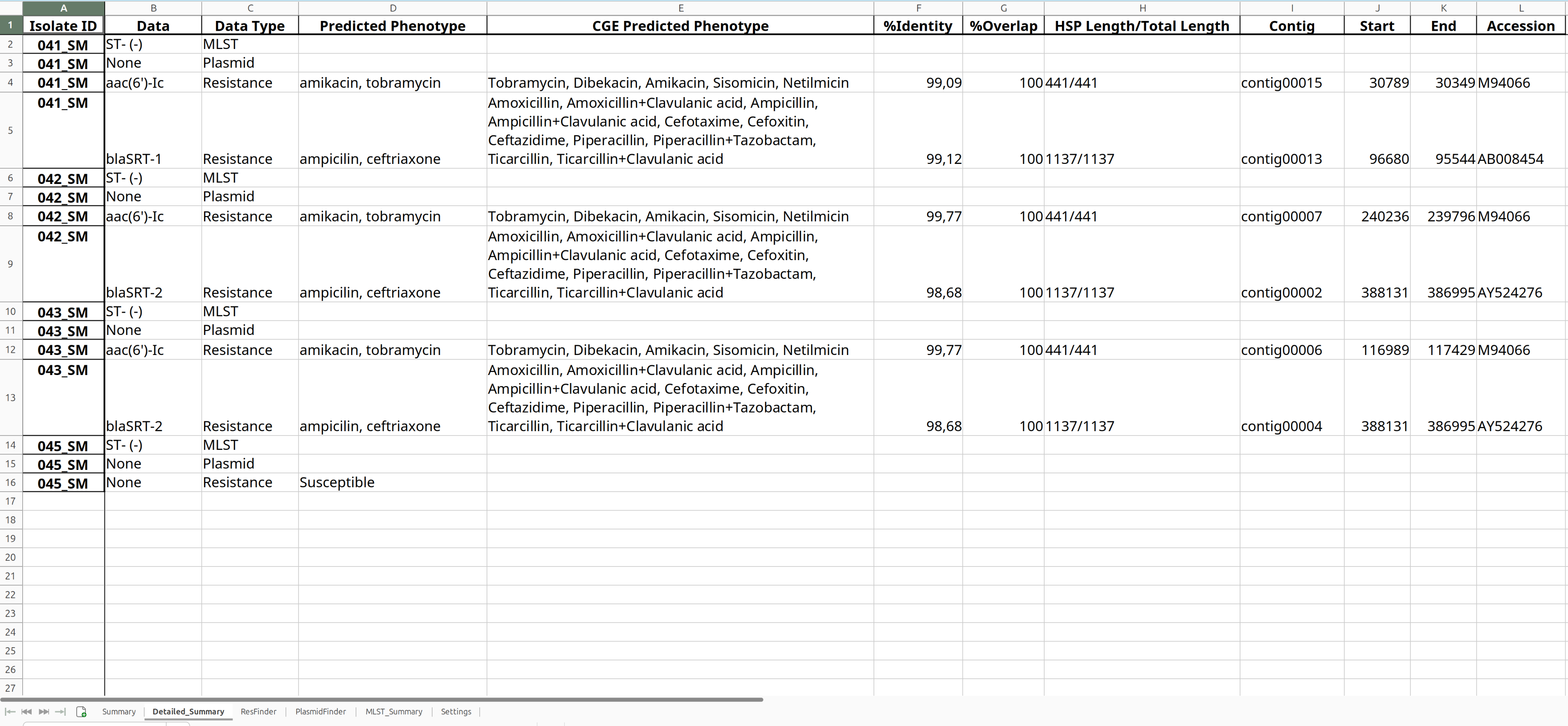
StarAMRStarAMR Tool with the following parameters:
CONTIGS collectionRun the tool and inspect the resulting reports.
The Excel output provides a convenient summary of the StarAMR results.
Download the file and inspect it.
ABRicateABRicate Tool with the following parameters:
Rename ABRicate output as AMR
ABRicate Summary Tool with the following parameters:
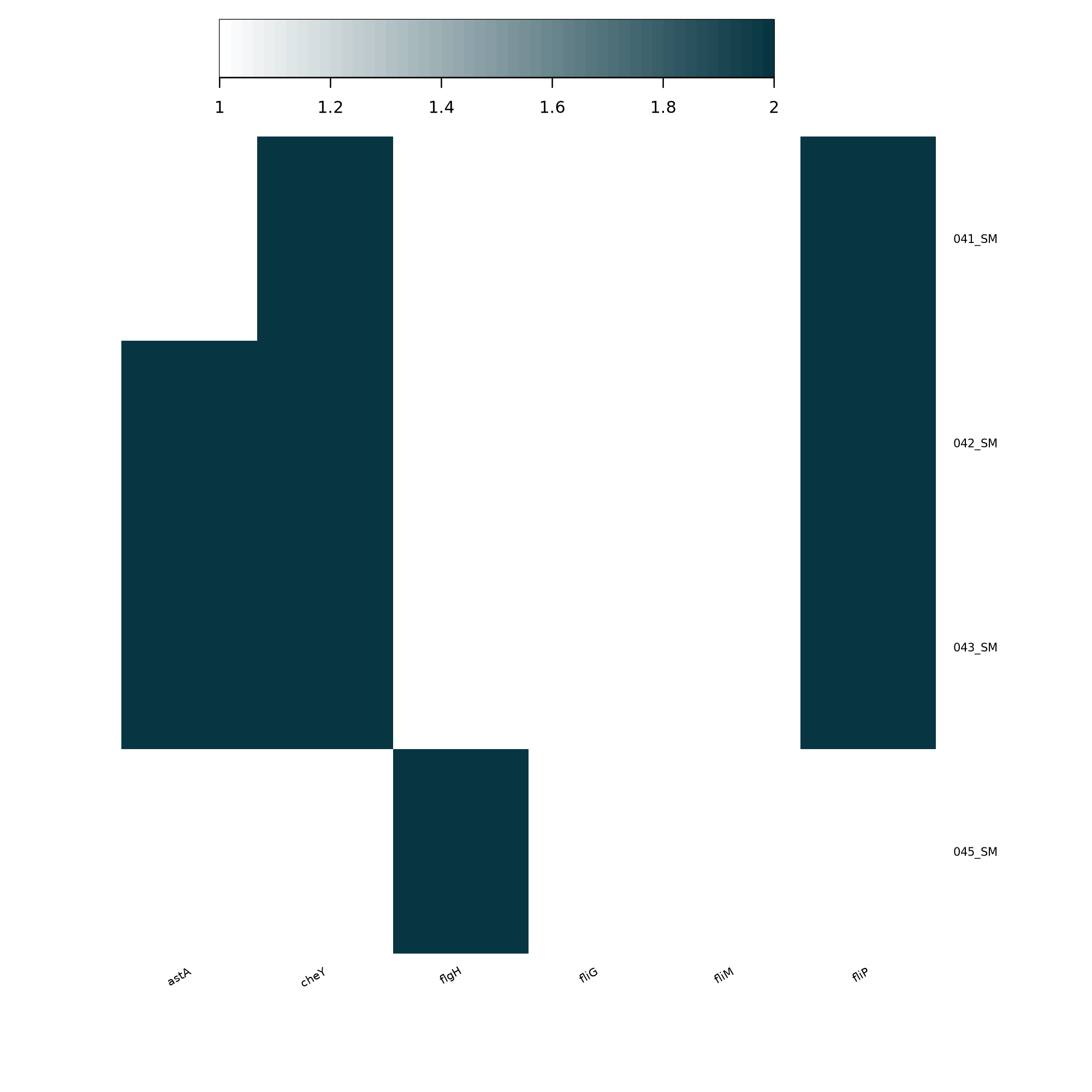
ABRicateABRicate Summary output as AMR summaryThe abricate summary output reports the percentage identity of each detected gene
for every genome analyzed.
| #FILE | NUM_FOUND | aac(6’)-Ic | aac(6’)_Serra | blaSRT | blaSRT-2 | oqxB30 | oqxB9 | tet(41) |
|---|---|---|---|---|---|---|---|---|
| 041_SM | 3 | . | 100.00 | 100.00 | . | . | 98.89 | . |
| 042_SM | 3 | 100.00 | . | . | 100.00 | . | 98.89 | . |
| 043_SM | 3 | 100.00 | . | . | 100.00 | . | 98.89 | . |
| 045_SM | 4 | . | 100.00 | 100.00 | . | 98.92 | . | 99.49 |
In this table:
. indicates absence of the geneFor heatmap visualization we do not need identity values, but only whether a gene is present or absent in each genome.
Therefore, the table must be converted into a binary matrix:
1 → gene present0 → gene absentExample of the required format (from Pathogen Identidification Tutorial :
| key | NP_231094 | NP_231099 | NP_231100 | NP_231101 | NP_231102 | NP_232418 | NP_232419 |
|---|---|---|---|---|---|---|---|
| SRR6871245 | 1 | 1 | 1 | 1 | 1 | 1 | 1 |
| SRR6871246 | 1 | 1 | 1 | 1 | 1 | 1 | 1 |
| SRR6871247 | 1 | 1 | 1 | 1 | 1 | 1 | 1 |
| SRR6871248 | 1 | 1 | 1 | 0 | 1 | 1 | 1 |
| SRR6871249 | 1 | 0 | 0 | 0 | 0 | 1 | 1 |
| SRR6871250 | 1 | 1 | 1 | 1 | 1 | 1 | 1 |
To generate this matrix:
key).NUM_FOUND column.. → 098.89, 100.00) → 1The resulting binary matrix can then be used to generate a gene presence/absence heatmap.
The resulting binary matrix can then be used to generate a gene presence/absence heatmap.
There are two possible ways to generate this matrix:
Using a spreadsheet editor
Download the abricate summary table, open it in a spreadsheet application (e.g. Excel), perform the conversion, save the modified table, and upload it back to Galaxy.
Using Galaxy tools
The same transformation can be performed directly in Galaxy using tools for text and tabular file manipulation.
Advanced Cut Tool with the following parameters:
Replace Tool with the following parameters:
Advanced Cut#FILEkey\d+\.\d{2}1Replace Tool with the following parameters:
Replace.0And, finally
heatmap2 Tool wit the followinf parameters:
Replace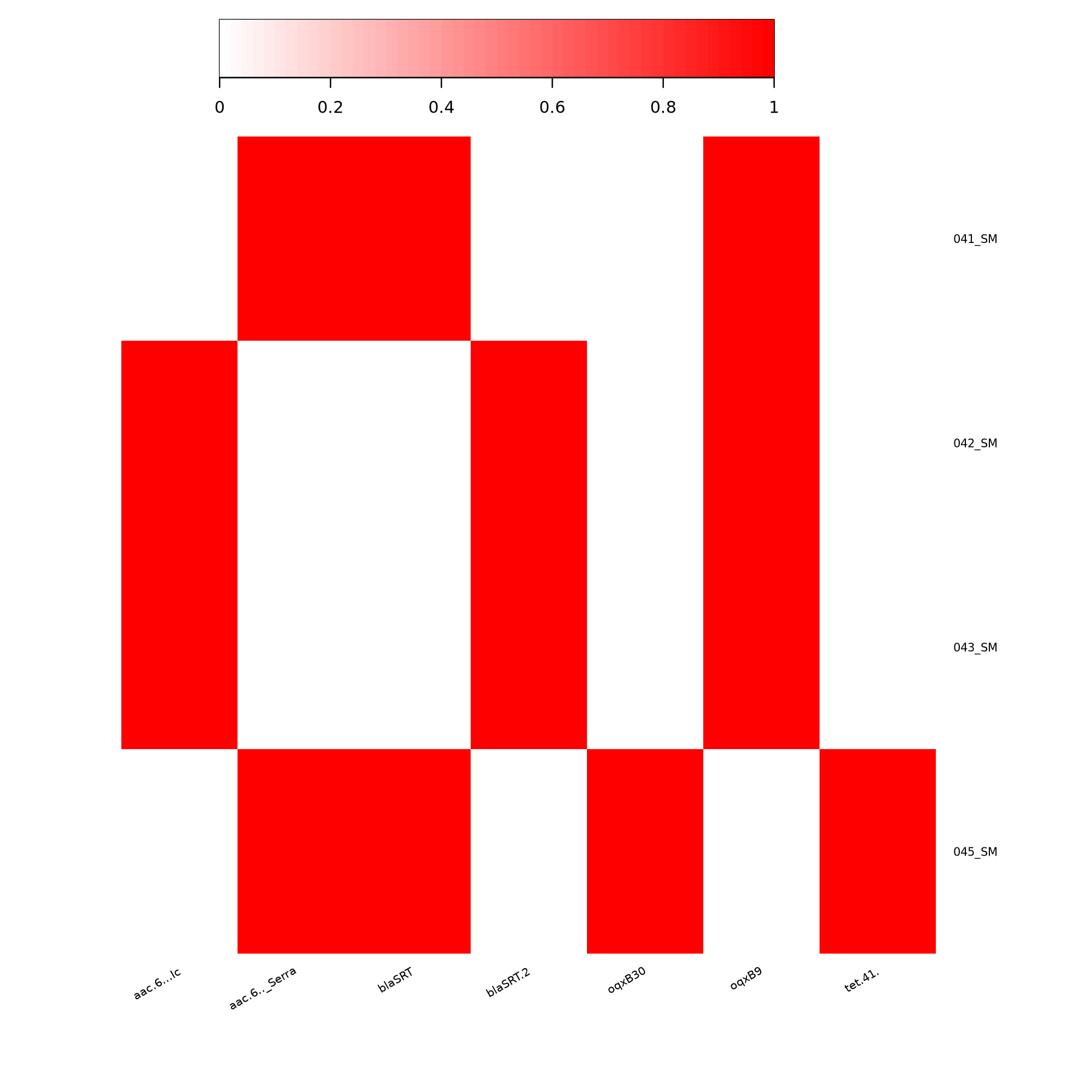
ABRicateABRicate Tool with the following parameters:
Rename ABRicate output as VFs
ABRicate Summary Tool with the following parameters:
ABRicateRename ABRicate Summary output as VFs summary
Prepare the Heatmap Input Matrix
MLST Tool with the following parameters:
In our dataset, the MLST tool does not return any results.
The analysis only works for species that have an available MLST scheme in the PubMLST database.
In this case, Serratia marcescens is not included among the typing schemes supported by the MLST database bundled with the tool.
Therefore, no allele matches or sequence types (ST) can be assigned.
This can be verified by running the MLST List tool, which displays the list of species for which MLST schemes are available in the database.
Note
MLST schemes for Serratia marcescens do exist in PubMLST, but they are not included in the version of the database distributed with the MLST tool used here.
In a command-line environment it is possible to manually add missing schemes by downloading the allele sequences and profile tables from the PubMLST REST API and updating the local MLST database.
However, this type of database customization is typically outside the scope of standard Galaxy workflows and requires direct access to the underlying system..
The MLST results obtained using the updated database have been uploaded to the shared Galaxy history
so that you can inspect and compare them with the other analyses performed in this tutorial.
Remember that the output file of the MLST tool is a tab-separated file containing:
| Column 1 | Column 2 | Column 3 | Column 4 | Column 5 | Column 6 | Column 7 | Column 8 | Column 9 | Column 10 |
|---|---|---|---|---|---|---|---|---|---|
| 041_SM | serratia | 595 | adk(142) | fumC(173) | gyrB(133) | icd(145) | mdh(131) | recA(128) | |
| 042_SM | serratia | 1406 | adk(174) | fumC(315) | gyrB(225) | icd(256) | mdh(398) | recA(220) | |
| 043_SM | serratia | 1406 | adk(174) | fumC(315) | gyrB(225) | icd(256) | mdh(398) | recA(220) | |
| 044_SM | ecloacae | 116 | dnaA(9) | fusA(4) | gyrB(14) | leuS(6) | pyrG(11) | rplB(4) | rpoB(6) |
| 045_SM | serratia | - | adk(1) | fumC(265) | gyrB(3) | icd(3) | mdh(2) | recA(3) | |
| 046_SM | serratia | - | adk(95) | fumC(117) | gyrB(108) | icd(269) | mdh(205) | recA(101) |
Pangenome analysis allows us to compare multiple genomes of the same species in order to identify:
For a detailed explanation of pangenome concepts and Roary parameters, refer to the dedicated tutorial: Pangenome Analysis Tutorial
Roary Tool with the following parameters:
- Individual gff files or a dataset collection: Collection
- Dataset collection to submit to Roary: GFF collection from Bakta
- In Additional Outputs
- Select Accessory binary genes in newick format
This option produces a phylogenetic tree based on the presence/absence patterns of accessory genes.
Roary generates a summary table describing the gene distribution across the analyzed genomes:
| Category | Definition | Genes |
|---|---|---|
| Core genes | (99% ≤ strains ≤ 100%) | 3648 |
| Soft core genes | (95% ≤ strains < 99%) | 0 |
| Shell genes | (15% ≤ strains < 95%) | 2793 |
| Cloud genes | (0% ≤ strains < 15%) | 0 |
| Total genes | (0% ≤ strains ≤ 100%) | 6441 |
Core genome (3648 genes)
Represents the conserved genetic backbone shared by all analyzed isolates.
Shell genes (2793 genes)
These genes are present in some but not all strains and represent the accessory genome, often associated with adaptation, mobile elements, or strain-specific traits.
Soft core and cloud genes
In this dataset, no genes fall into these intermediate categories.
The total number of genes across the pangenome is 6441
The core genome defines the species, while the accessory genome explains the diversity between strains.
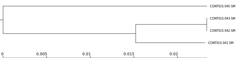
If the option Accessory binary genes in newick format was selected, Roary generates a tree based on the presence/absence patterns of accessory genes.
This tree can be visualized using the Newick Display tool.
Newick Display
Accessory binary genes (newick) produced by RoaryThis tree represents similarity in gene content between genomes.
Genomes that cluster together in this tree share a similar set of accessory genes, which may include:
However, this tree does not represent the evolutionary history of the strains, because accessory genes can be exchanged through horizontal gene transfer.
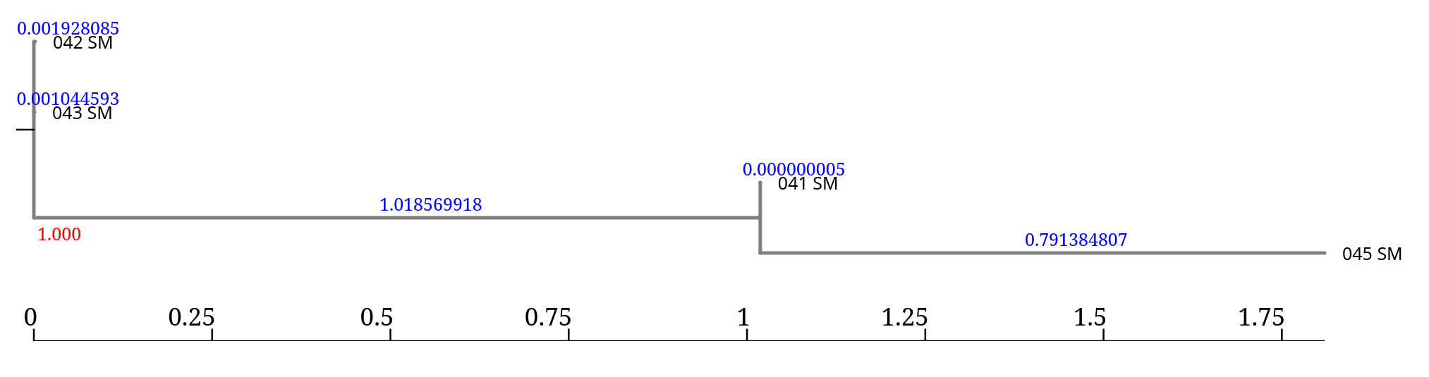
The accessory genome tree generated by Roary is stored in Newick format.
(042_SM:0.001928085,043_SM:0.001044593, (041_SM:0.000000005,045_SM:0.791384807)1.000:1.018569918);
041_SM, 045_SM): represent branch length) represent branch supportInterpretation:
041_SM and 045_SM form a cluster (sister taxa)1.000 indicates 100% support for this groupingIn this case, the tree indicates that:
Remember:
Consider this part of the tree:
(041_SM:0.000000005,045_SM:0.791384807)1.000:1.018569918
Here we have three branch length values:
| Genome / Node | Branch length |
|---|---|
| 041_SM | 0.000000005 |
| 045_SM | 0.791384807 |
| internal node | 1.018569918 |
Branch lengths are distance values, not percentages.
So in relative terms:
041_SM is almost identical to its ancestor node045_SM is more divergent1.018 indicates the largest separation between clustersIn an accessory genome tree, branch length reflects differences in gene content, not evolutionary time.
Therefore:
Branch length values are meaningful only when compared within the same tree, not across different analyses.
The tree generated by Roary is stored in Newick/NHX format.
To visualize and explore it interactively, we can use the online tool iTOL (Interactive Tree Of Life).
Download the file Accessory binary genes (newick) produced by Roary from your Galaxy history.
Open the iTOL website: https://itol.embl.de
Click Upload Tree.
Upload the downloaded .nwk / .nhx file.
Once uploaded, iTOL automatically renders the tree.
You can then:
iTOL is particularly useful for exploring larger trees and preparing publication-quality figures.
To infer the evolutionary relationships between the isolates, we must instead use the core genome alignment produced by Roary.
Roary generates the file:
core_gene_alignment.aln
This multiple sequence alignment can be used to build a phylogenetic tree using tools such as:
RAxMLIQ-TREEFastTreeThese tools reconstruct a tree based on sequence evolution of the conserved core genes, providing a more accurate representation of the phylogenetic relationships between strains.
Running RAxML on the core genome alignment produces several output files:
| Output | Description |
|---|---|
| Info | Summary of the analysis parameters and run statistics (model used, number of sites, likelihood scores). |
| Log | Detailed log of the optimization process performed during the ML search. |
| Parsimony Tree | Starting tree generated using the maximum parsimony method. This tree is used as an initial guess for the ML search. |
| Result | One of the trees obtained during the ML optimization process. |
| Best-scoring ML Tree | The final phylogenetic tree with the highest likelihood score. This is the tree typically used for interpretation and visualization. |
In practice:
Newick DisplayThis tree represents the phylogenetic relationships between the isolates based on the core genome alignment.
The Best-scoring ML Tree generated by RAxML represents the phylogenetic relationships between the isolates based on the alignment of core genes.
Because core genes are conserved and typically inherited vertically, this tree approximates the evolutionary history of the strains.
When interpreting a phylogenetic tree, focus on three main elements.
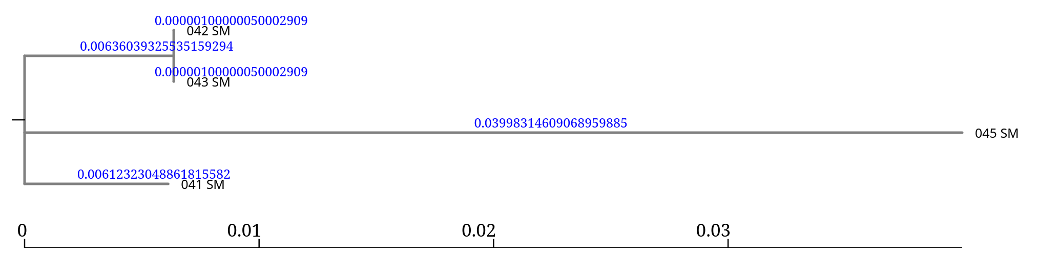
This tree therefore describes the evolutionary relationships between the isolates based on their conserved genome backbone.
Running IQ-TREE on the core genome alignment generates several output files.
| Output | Description |
|---|---|
| BIONJ Tree | Initial tree built using the BIONJ distance method. This tree serves as a starting point for the maximum likelihood optimization. |
| MaxLikelihood Tree | The maximum likelihood phylogenetic tree inferred from the alignment. This is the tree used for interpretation and visualization. |
| MaxLikelihood Distance Matrix | Pairwise genetic distance matrix between genomes derived from the alignment. |
| Occurrence Frequencies in Bootstrap Trees | Table summarizing how frequently each split appears across bootstrap replicates, used to calculate branch support. |
| Report and Final Tree | Detailed report describing the analysis, parameters used, likelihood scores, and summary of the final tree inference. |
In practice, the most important file for visualization is: MaxLikelihood Tree. This file can be opened withNewick Display
and represents the phylogenetic relationships between the isolates based on the core genome alignment.
When running FastTree on the core genome alignment, with Nucleotide option, the tool produces a single output:
| Output | Description |
|---|---|
| Tree | The inferred phylogenetic tree in Newick format. |
Unlike tools such as IQ-TREE or RAxML, which generate multiple intermediate files and reports, FastTree outputs only the final tree.
FastTree is designed to infer trees very quickly, even for large datasets.
Advantages:
However, it is generally considered less rigorous than full maximum likelihood methods such as IQ-TREE or RAxML.
For exploratory analyses or large datasets, FastTree is often sufficient, while IQ-TREE or RAxML are preferred for more robust phylogenetic inference.
Two complementary views of genomic diversity are obtained:
| Tree type | Based on | Biological meaning |
|---|---|---|
| Core genome tree | Sequence alignment of conserved genes | Evolutionary relationships |
| Accessory genome tree | Presence/absence of accessory genes | Functional genomic similarity |
Another common approach to infer phylogenetic relationships between bacterial isolates is SNP-based phylogeny.
Instead of comparing full gene sequences, this method focuses only on single nucleotide polymorphisms (SNPs) across the genomes.
Because SNPs capture very small genetic differences, this approach provides very high resolution and is widely used in:
The general workflow for SNP-based phylogeny includes several steps:
Reference genome selection
A suitable reference genome is chosen for the species under study.
Read mapping
Sequencing reads are aligned to the reference genome.
Variant calling
SNPs are identified by comparing each isolate to the reference genome.
SNP filtering
Low-quality or unreliable variants are removed.
Core SNP alignment
SNP positions shared across all isolates are extracted to create an alignment.
Phylogenetic inference
A phylogenetic tree is reconstructed using tools such as:
The resulting tree represents the phylogenetic relationships between isolates based on nucleotide differences across the genome.
Because SNPs capture very small genetic differences, SNP-based phylogenies provide high-resolution comparisons between strains.
Running each step separately can be complex.
For bacterial genomes, the pipeline can be simplified using Snippy.
Snippy is a tool specifically designed for rapid SNP detection in bacterial genomes.
It automatically performs several steps of the workflow:
This greatly simplifies the analysis and reduces the number of tools required.
The output generated by Snippy can then be used to build a core SNP alignment, which serves as input for phylogenetic inference with tools such as IQ-TREE or RAxML.
Because of its simplicity and reliability, Snippy is widely used in bacterial genomics and outbreak analysis.
Snippy tool with the following parameters:
snippy-core tool with the following parameters:
SnippyRaxml or IQ-Tree with Core Alignment Fasta from snippy-coreSnippy has taken the reads and:
mapped them against the reference using BWA MEM,
looked through the resulting BAM file and found differences using some fancy Bayesian statistics (Freebayes),
filtered the differences for sensibility and finally checked what effect these differences will have on the predicted genes and other features in the genome.
It produces quite a bit of output, there can be up to 10 output files.
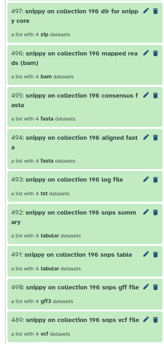
snps vcf file: The final annotated variants in VCF format
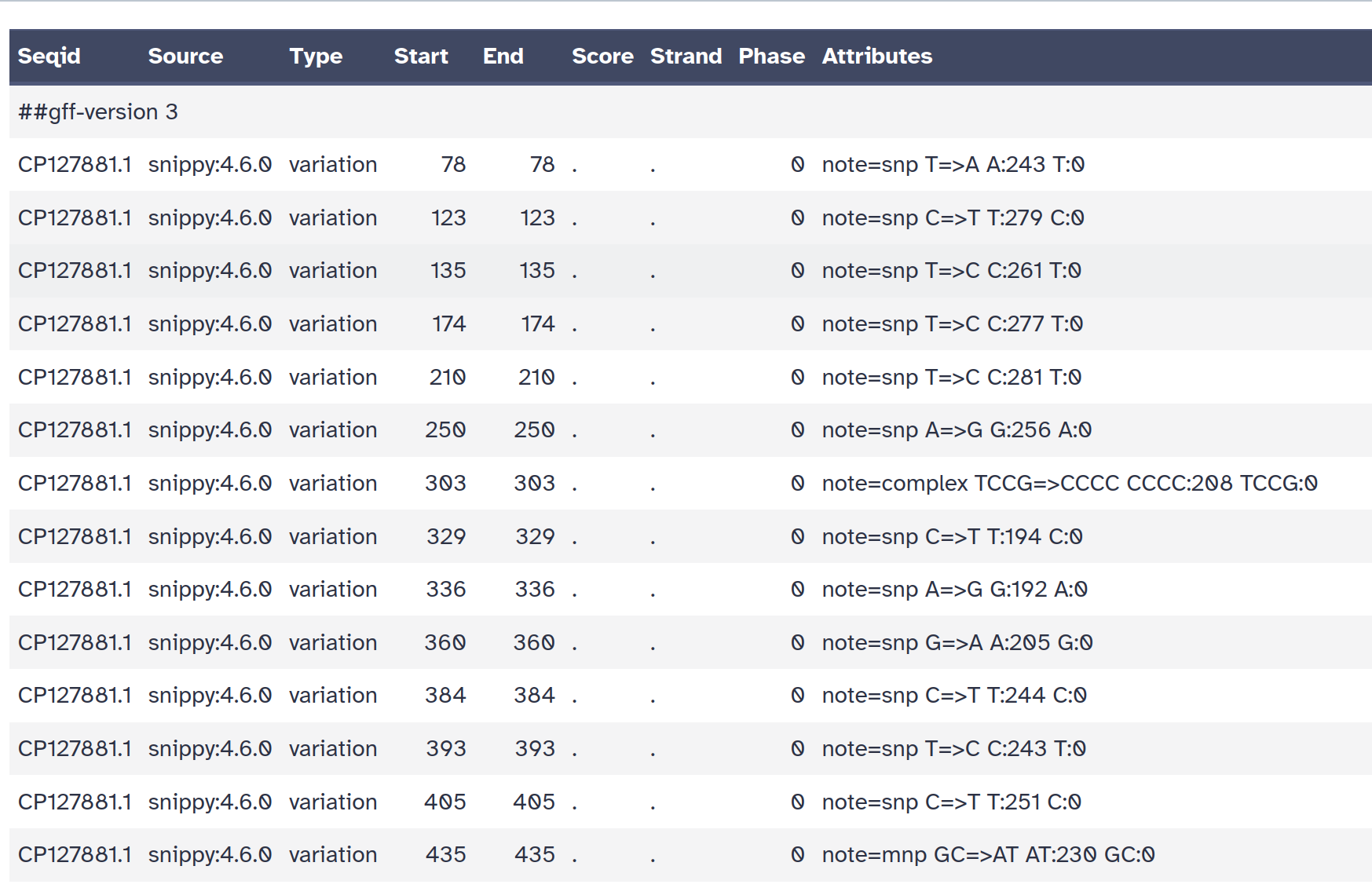
snps gff file: The variants in GFF3 format
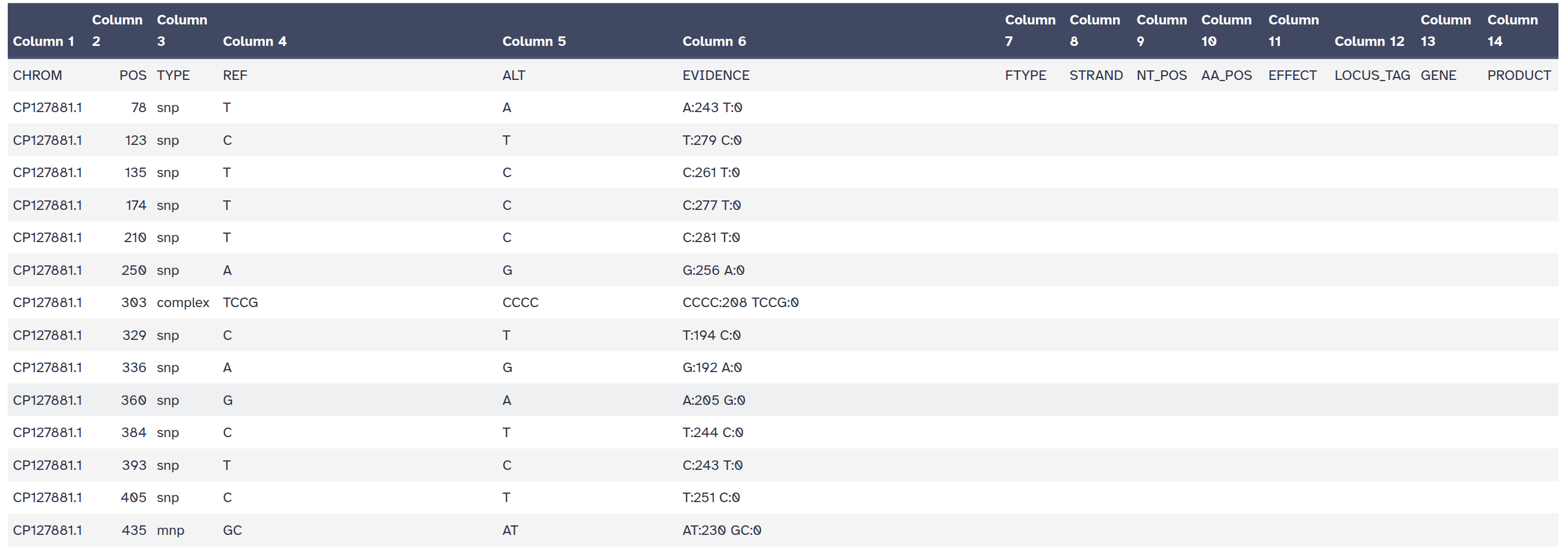
snps table: A simple tab-separated summary of all the variants
snps summary: A summary of the SNPs called
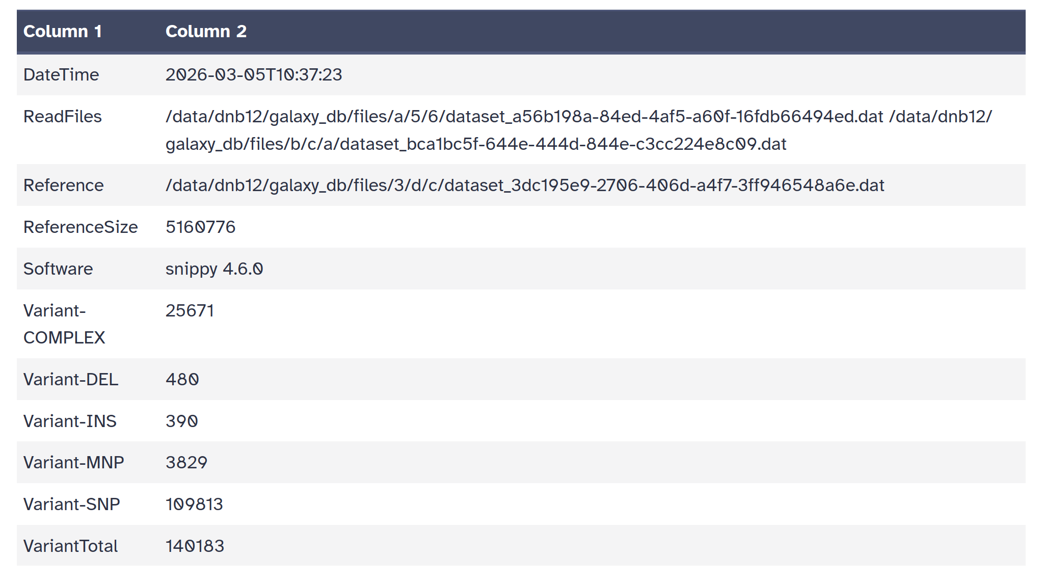
log file: A log file with the commands run and their outputs
aligned fasta: A version of the reference but with - at position with depth=0 and N for 0 < depth < –mincov (does not have variants)
consensus fasta: A version of the reference genome with all variants instantiated
mapping depth: A table of the mapping depth
mapped reads bam: A BAM file containing all mapped reads
outdir: A tarball of the Snippy output directory for input into snippy-core
| ID | LENGTH | ALIGNED | UNALIGNED | VARIANT | HET | MASKED | LOWCOV |
|---|---|---|---|---|---|---|---|
| 041_SM | 516077 | 64372 | 72476 | 7318 | 183 | 171105 | 9019675 |
| 042_SM | 516077 | 64416 | 61972 | 5011 | 176 | 117710 | 018436 |
| 043_SM | 516077 | 64417 | 25172 | 5218 | 176 | 023790 | 017517 |
| 045_SM | 516077 | 64515 | 21962 | 8970 | 175 | 989862 | 015725 |
| Reference | 516077 | 65160 | 77600 | 0000 | 0 | 0 | 0 |
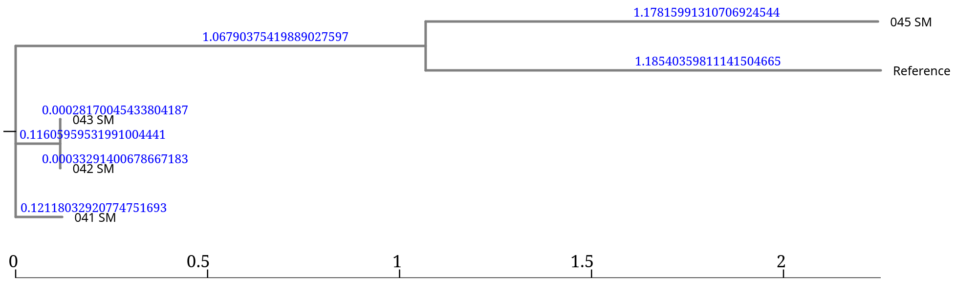
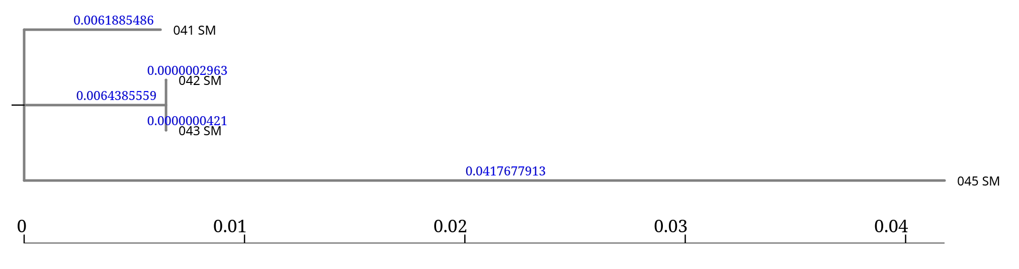
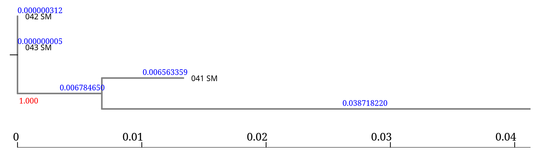
From the topology we observe:
Branch lengths represent the number of nucleotide differences detected across the genome.
Very small values (e.g. 0.00028) indicate nearly identical genomes,
while larger values indicate greater genetic divergence.
In this tree, the branch lengths associated with 045_SM and the reference are much larger, suggesting that this isolate is much more divergent from the other samples.
Extremely long branches in SNP phylogenies may indicate a distant lineage, an unsuitable reference genome, or potential issues in the assembly or mapping.
Average Nucleotide Identity (ANI) is a metric used to measure the genomic similarity between two microbial genomes.
It calculates the average nucleotide identity of homologous genomic fragments shared between the genomes.
ANI is widely used for species identification in prokaryotes and has largely replaced traditional DNA–DNA hybridization methods.
A commonly accepted rule is:
| ANI value | Interpretation |
|---|---|
| ≥ 95–96 % | genomes belong to the same species |
| 90–95 % | closely related species |
| < 90 % | different species |
ANI can be computed using FastANI, a fast alignment-based method designed for large-scale microbial genome comparisons.
FastANI works by:
The tool reports:
ANI values between the isolates and the reference genome range between 95.1% and 95.4%.
Since the commonly accepted species threshold is 95–96% ANI, all isolates are consistent with belonging to Serratia marcescens.
Although isolate 045_SM appears more divergent in the phylogenetic trees, the ANI analysis confirms that it still falls within the same species boundary.
Phylogenetic distance does not necessarily imply species divergence.
An isolate may appear phylogenetically distant, yet still belong to the same species, as confirmed by ANI analysis.
While phylogenetic trees describe evolutionary relationships between genomes, population genomics approaches can identify genomic clusters or lineages within a species.
One tool commonly used for this purpose is PopPUNK
(POPulation Partitioning Using Nucleotide Kmers).
PopPUNK is typically applied to large genomic datasets (tens to thousands of genomes).
| Taxon | Cluster |
|---|---|
| CONTIGS_042_SM | 1 |
| CONTIGS_043_SM | 1 |
| CONTIGS_041_SM | 2 |
| CONTIGS_045_SM | 3 |
From the analyses performed in this tutorial we can draw several conclusions.
Two samples (044 and 046) showed clear evidence of contamination and were excluded from downstream analyses.
The remaining four genomes produced high-quality assemblies consistent with the expected genome size and GC content of Serratia marcescens.
AMR analysis revealed a small set of resistance genes shared across the isolates, with minor variation between strains.
Pangenome analysis identified a core genome of 3648 genes and a substantial accessory genome contributing to strain diversity.